the Creative Commons Attribution 4.0 License.
the Creative Commons Attribution 4.0 License.
 | 03 Jul 2018
Background noise estimation of the geomagnetic signal
Xiuyi Yao
Suqin Zhang
Yuntian Teng
Dongmei Yang
A fast Fourier transform was applied to fit the geomagnetic diurnal variation. Fitting results showed that when the polynomial degree was greater than 160, the residual error was close to 0 nT. White noise is the main component of the residual error when the polynomial degree was greater than 160, so this method was adopted to calculate the background noise of the geomagnetic field. Spectrum analysis further demonstrated that the noise estimation result is reliable.
- Article
(4620 KB) -
Supplement
(67876 KB) - BibTeX
- EndNote


The geomagnetic field is critical for solar activity monitoring, space weather detection, and some investigations into crustal motions that lead to geomagnetic field changes (Chapman and Bartels, 1940; Campbell, 1997). Because of the various factors influencing the geomagnetic field, the sources of geomagnetic signal noise are also diverse. According to previous studies, the noise of the geomagnetic signal can be divided into two types (Ren, 2006). Variable noise changes over time and comes from fluctuations within conductive fault zones or from instability within the observation environment, which acts as an antenna to couple with the external geomagnetic field. Background noise is more stable; it originates within a stable observation environment and from instrumental responses, such as thermal noise and other electronic noise. The noise within geomagnetic data plays an important role in evaluating the quality of geomagnetic data and also has an impact on scientific research (Yao et al., 1995).
Historically, variable noise in geomagnetic observations was calculated by first difference. In previous studies, some results such as temporal characteristics, spatial distribution features, and influencing factors of variable noise were achieved (Yan et al., 2013; Wang et al., 2015). According to previous research results, the intensity of variable noise is extremely weak and usually lower than an instrumental resolution of 0.1 nT. This suggests that background noise may be the main component of geomagnetic noise. However, previous research also showed that it is difficult to calculate background noise quantitatively because of the inseparability of the geomagnetic signal and noise. In seismology, signal-to-noise ratio (SNR) estimation on noisy data is mainly obtained through the energy superposition method, spectrum analysis, or power spectrum calculation (Zhang et al., 2009). Because of the nonstationarity of the geomagnetic field, these methods are not suitable for geomagnetic SNR estimation. Zhu et al. (2012, 2013) and Wang et al. (2015) applied principal component analysis (PCA) to suppress noise in airborne electromagnetic data. Nevertheless, PCA needs observation data from at least three groups at the same observatory, which is improbable for most geomagnetic observatories. Jiang et al. (2013) used maximum likelihood estimation to calculate geomagnetic noise through multiple iterations. However, many previous studies have suffered from deficiencies in testing.
In this paper, the diurnal geomagnetic data were fitted through a fast Fourier transform (FFT), and then the residual error between original and fitted data was obtained to estimate the background noise of geomagnetic data. In previous studies, researchers applied an FFT to geomagnetic diurnal variation (Han et al., 2009; Zhao et al., 2014; Koch and Kuvshinov, 2015; Yamazaki and Maute, 2017). However, almost all of them focused on the Sq diurnal variation, so the polynomial degree is no greater than 6. In general, when geomagnetic disturbances are absent, the first four harmonics are sufficient to capture most of the variability in a daily record of the geomagnetic field. We suggest analysis of geomagnetic diurnal variation by the use of FFT with a degree of 250; the residual error may represent changes in background noise. The testing result showed that this approach to estimate background noise in geomagnetic data is effective.
FFT is the most widely used method of spectrum analysis. Any periodic signal can be decomposed into several components such as first harmonics (T), second harmonics (T∕2), third harmonics (T∕3) and more (Cooley and Tukey, 1965) through the FFT.
A time-series signal can be expressed as a function of sine and cosine as follows:
where a(m) and b(m) are coefficients of sine and cosine functions, respectively. λl is a function of l, and l indicates the sequence number of the data series. M represents the total number of data point.
Normal daily variation in the geomagnetic field mainly comprises the first six harmonic components (Fig. 1); these components represent signals of period 24, 12, 8, 6, 4.8, and 4 h, and results of higher degree (N) achieve closer fits.


The background noise of the geomagnetic vertical component (Z) is more complex because this component is more susceptible to the change in observation environment. Furthermore, in order to reduce the influence of the external geomagnetic field, data from the quietest days of 2013 were chosen and an FFT was applied to fit them for the 10th–250th harmonic components. The residual error (Error in Eq. 3) between original data and fitted data was calculated by as follows:
Here, ff(l) represents the original geomagnetic data, and f(l) indicates the fitted data through FFT. The sampling rate of the original data is 1 Hz, so the total number (M) of samples in 1 day is 86 400. As displayed in Fig. 2, the residual error is less than 1.0 nT when the polynomial degree is greater than 10, and smaller residual errors generally correlated with larger polynomial degrees. When the polynomial degree is greater than 160, the residual error approaches 0 nT. Based on previous analysis results, it is reasonable to assume that the fitted data of the 160th degree could represent the original signal in which background noise is not contained.
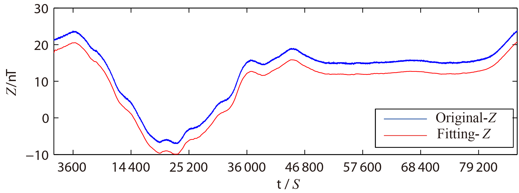
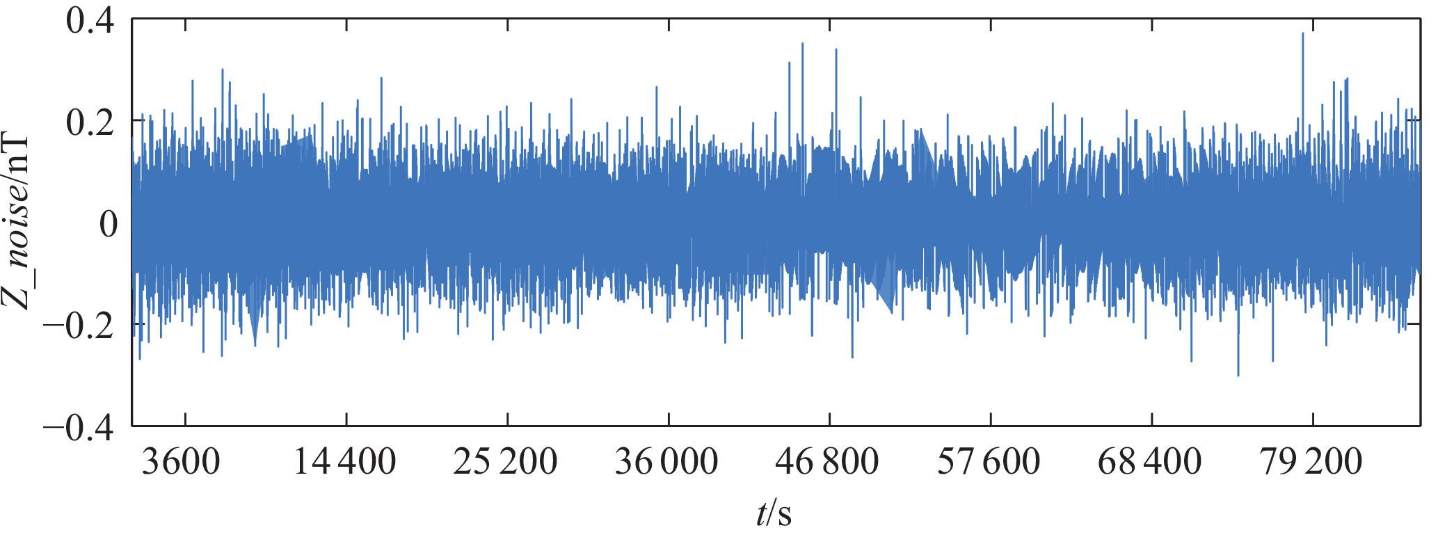
Figure 3 shows the original signal and the FFT-fitted data with a polynomial degree of 160 on 29 May 2013 at the LYH (37.40 N, 114.70 E) observatory as an example; a constant is added between them for comparison. The fitted curve is almost identical to the original curve, though the fitted curve is smoother. This implies that the background noise of the geomagnetic signal could be estimated through FFT fitting with a polynomial degree of 160. The background noise of the geomagnetic vertical component is marked as Z_noise and is obtained from Eq. (4). ff(l) in Eq. (4) represents the original geomagnetic data, and f(l) indicates the fitted data through FFT with a polynomial degree of 160. Figure 4 shows the estimated background noise on 29 May 2013 at the LYH observatory as an example. It is randomly distributed between −0.2 and 0.2 nT with a mean value of 0 nT.
White noise is a random signal with a mean value of 0. Based on the characteristics of Z_noise obtained from Fig. 4, we think the main composition of Z_noise may be white noise, which associated with the geomagnetic instrument and the observation environment.
Standard white noise is a random signal with a mean value of 0, and its autocorrelation function is close to 0 when the lag (τ) is not equal to 0. To confirm that the main composition of Z_noise is white noise, the autocorrelation function of Z_noise is calculated from Eq. (5).
Rτ is the autocorrelation function of signal, E is the expected value operator, Xt indicates data of Z_noise at time t, μ and σ2 represent the mean value and variance of Z_noise, and τ is the lag. Figure 5 shows the autocorrelation function of background noise on 29 May 2013 at the LYH observatory. The autocorrelation function of Z_noise clearly reaches up to 1 when τ=0 and is close to 0 when τ≠0, the same as the autocorrelation of white noise. Therefore, it is demonstrated that the main composition of Z_noise is white noise, and the background noise of the Z component of the geomagnetic field (Z_noise) could be obtained through FFT fitting with a polynomial degree of 160.
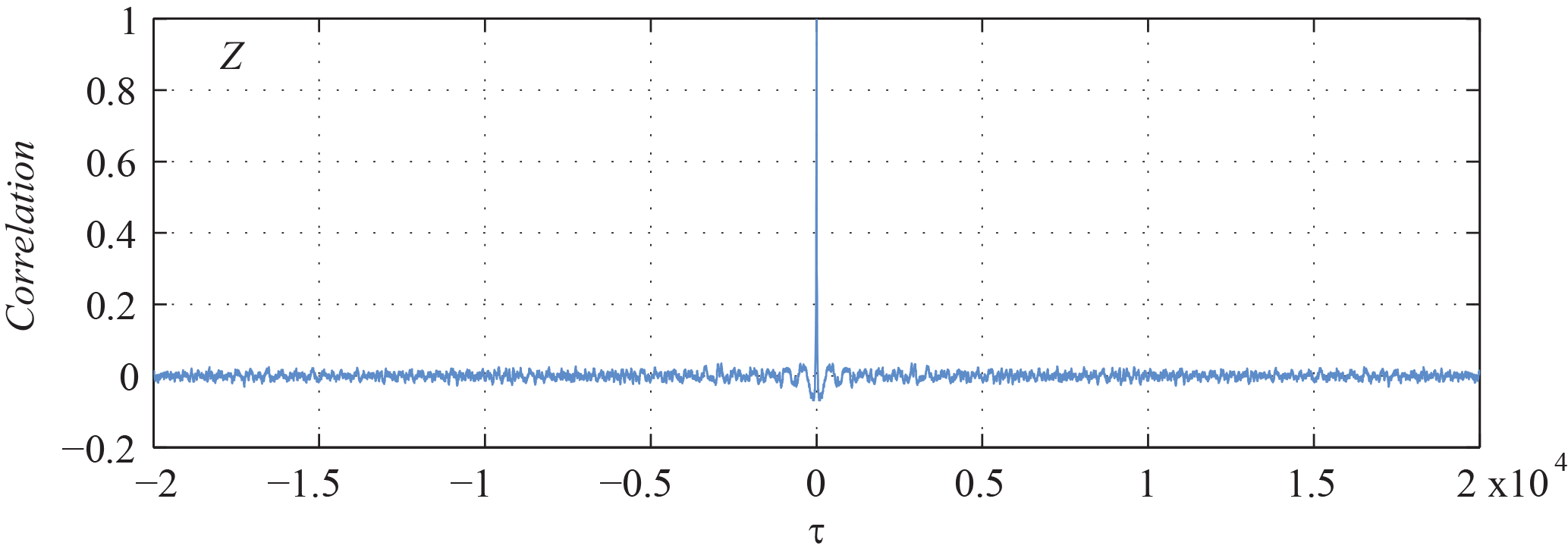
Figure 5Autocorrelation function of background noise in the Z component on 29 May 2013 at LYH.
The SNR of the geomagnetic signal can be calculated as Eq. (6) when background noise is obtained. The result shows that the SNR of geomagnetic data from the LYH observatory is about 47.
To contrast the original geomagnetic data and the noise-free geomagnetic data, their frequency spectra were analyzed. Waveforms of the geomagnetic vertical component (Z) during each interval of 30 min were subjected to FFT spectrum analysis as follows:
Here, , and R(u, ν) and I(u, ν) indicate the real and imaginary parts of FFT result, respectively. F(u, ν) represents the amplitude of the FFT spectrum.
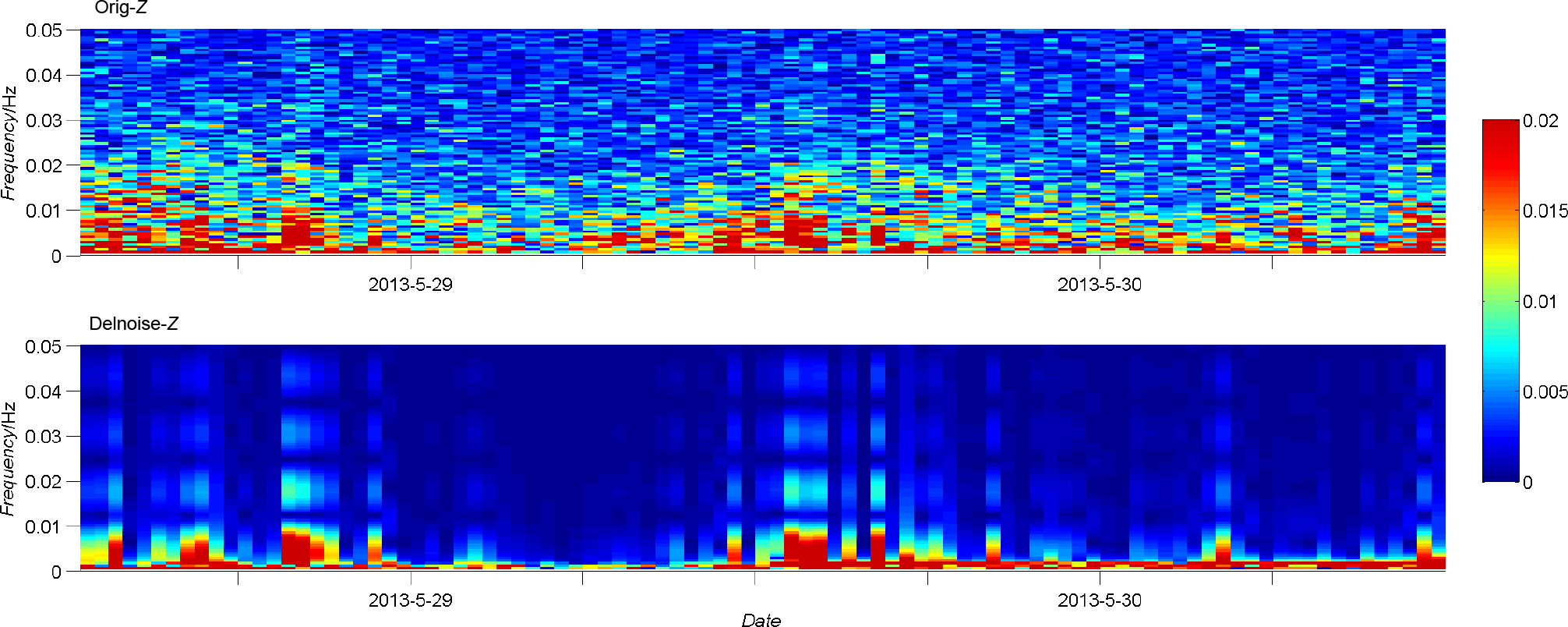
The upper panel of Fig. 6 shows amplitude spectrum of original signal on 29 and 30 May 2013 at the LYH observatory. The amplitude spectrum of the original data is clearly more irregular; its background noise can be seen as scattered points in the spectrum, and the intensity of these points is not related to frequency or time. Because of the influence of background noise, the amplitude spectrum of the original geomagnetic signal does not show any significant changes over this interval. The bottom panel of Fig. 6 represents the amplitude spectrum of the geomagnetic data after removing background noise. It is different from the upper panel. Irregularly scattered points representing background noises are removed almost completely, and, as a result, the amplitude spectrum is more regular and informative. From the bottom panel of Fig. 6, some significant characteristics are obtained. First, geomagnetic energy changes with frequency: the lower the frequency of the signal is, the higher the geomagnetic energy. Second, geomagnetic activity in each 30 min block is different. In the first 24 half hours of 29 May 2013 and the first 24 half hours of 30 May 2013 the geomagnetic activity is more intense than any others. In contrast, these characteristics are not immediately obvious in the amplitude spectrum of the original data, implying that FFT filtering is an effective method for geomagnetic background noise estimation.
The background noise of the geomagnetic signal can be obtained through FFT filtering with a polynomial degree of 160 on the vertical component (Z) during the quietest days. The main conclusions are summarized as follows:
-
The residual error between FFT-filtered data and the original signal approaches 0 nT as the polynomial degree is greater than 160, and it has been confirmed that a residual error with a degree of 160 could represent the background noise of the geomagnetic signal.
-
Geomagnetic background noise is a random signal distributed between −0.2 and 0.2 nT.
-
The autocorrelation function of background noise showed that it reaches up to 1.0 when lag (τ) is 0 and is close to 0 in other cases, which confirms that white noise is the main component of geomagnetic background noise.
-
Spectrum analysis further confirms that FFT filtering is an effective method for geomagnetic background noise estimation, and some geomagnetic changes are more remarkable after filtering.
FFT-filtered data with a polynomial degree greater than 160 could represent the original geomagnetic signal with a period of less than 540 s. Any signal with a period of less than 540 s in the original data will be removed completely in the filtered data. To avoid overprocessing, data from the quietest days were chosen, avoiding short-period variations such as pulsations or geomagnetic bays. In addition, because the vertical component (Z) contains more noise information than other components and is not as susceptible to the external geomagnetic field, it was chosen as the analysis object in this paper. Because the main factors influencing background noise are the local observation environment and the instrumental response, the geomagnetic background noise at different observatories differs. For any one particular observatory, background noise is usually nearly invariable due to the stability of the observation environment and the instrument condition.
Geomagnetic data of observatories can be obtained from http://www.geomag.org.cn/.
The supplement related to this article is available online at: https://doi.org/10.5194/gi-7-189-2018-supplement.
The authors declare that they have no conflict of interest.
This work was supported by a project of Science for Earthquake Resilience of
China (XH18041Y) and The National Natural Science Foundation of China
(41504129). We thank the Geomagnetic Network of China for providing
geomagnetic data of observatories.
Edited by: Lev Eppelbaum
Reviewed by: Xudong Zhao and one anonymous referee
Campbell, W. H.: Introduction to Geomagnetic Field, Cambridge University Press, New York, 10–40, 1997.
Chapman, S. and Bartels, J.: Geomagnetism, Oxford Clarendon Press, New York, 12–30, 1940.
Cooley, J. W. and Tukey, J. W.: An Algorithm for the Machine Calculation of Complex Fourier Series, Math. Comput., 19, 297–301, https://doi.org/10.1090/S0025-5718-1965-0178586-1, 1965.
Han, P., Huang, Q. H., and Xiu, J. G.: Principal component analysis of geomagnetic diurnal variation associated with earthquakes: case study of the M6.1 Iwate-kenNairiku Hokubu earthquake, Chinese J. Geophys.-Ch., 52, 1156–1563, https://doi.org/10.3969/j.issn.0001-5733.2009.06.001, 2009.
Jiang, C., Zhong, G. P., Zhang, F. L., Zhang, G. S., and Wu, C. Z.: Study on noise characteristics of time series of geomagnetic observation on Jilin, Earthquake Research in Shanxi, 2, 8–10, https://doi.org/10.3969/j.issn.1000-6265.2013.02.003, 2013.
Koch, S. and Kuvshinov, A.: 3-D EM inversion of ground based geomagnetic Sq data, Results from the analysis of Australian array (AWAGS) data, Geophys. J. Int., 200, 1284–1296, https://doi.org/10.1093/gji/ggu474, 2015.
Ren, X. X.: Study on the noise in simultaneous geomagnetic difference data caused by the effect of Sq local-time variation, Acta Seismologica Sinica, 28, 85–90, https://doi.org/10.3321/j.issn:0253-3782.2006.01.011, 2006.
Wang, J., Hu, X. J., Luo, N., Li, X. S., Wang, L. B., Song, Z., and Chang, G. P.: The analysis of reference background noise of fluxgate magnetometer GM4 at Hongshan seismic station, Seismological and Geomagnetic Observation and Research, 36, 105–109, https://doi.org/10.3969/j.issn.1003-3246.2015.03.019, 2015.
Wang, L. Q., Li, B. B., Lin, J., Xie, B., Wang, Q., Cheng, Y. Q., and Zhu, K. G.: Noise removal based on reconstruction of filtered principal component, Chinese J. Geophys.-Ch., 58, 2803–2811, https://doi.org/10.6038/cjg20150815, 2015.
Yamazaki, Y. and Maute, A.: Sq and EEJ-Areview on the daily variation of the geomagnetic field caused by ionospheric dynamo current, Space Sci. Rev., 206, 299–405, https://doi.org/10.1007/s11214-016-0282-z, 2017.
Yan, J. M., Zhang, L. E., Cheng, C. J., He, Y. F., and Yang, X.: The interference factor on background noise of the geomagnetic data in Taiyuan geomagnetic observatory, Seismological and Geomagnetic Observation and Research, 34, 135–140, https://doi.org/10.3969/j.issn.1003-3246.2013.05/06.022, 2013.
Yao, T. Q., Fan, G. H., and Gu, Z. W.: The use of adaptive filter for noise processing on geomagnetic data, Seismological and Geomagnetic Observation and Research, 16, 12–18, 1995.
Zhang, J. H., Zang, S. T., Zhou, Z. X., Wang, J., Shan, L. Y., Xu, H., Fu, J. R., Yu, H. C., and Bu, C. C.: Quantitative computation and comparison of S/N ratio in seismic data, Oil Geophysical Prospecting, 44, 481–486, https://doi.org/10.13810/j.cnki.issn.1000-7210.2009.04.021, 2009.
Zhao, X. D., Yang, D. M., He, Y. F., Yu, P. Q., Liu, X. C., Zhang, S. Q., Luo, K. Q., and Hu, X. J.: The study of Sq equivalent current during the solar cycle, Chinese J. Geophys.-Ch., 57, 3777–3788, https://doi.org/10.6038/cjg20141131, 2014.
Zhu, K. G., Ma, M. Y., Che, H. W., Yang, E. W., Ji, Y. J., Yu, S. B., and Lin, J.: PC-based artificial neural network inversion for airborne time-domain electromagnetic data, Appl. Geophys., 9, 1–8, https://doi.org/10.1007/s11770-012-0307-7, 2012.
Zhu, K. G., Wang, L. Q., Xie, B., Wang, Q., Cheng, Y. Q., and Lin, J.: Noise removal for airborne electromagnetic data based on principal component analysis, The Chinese Journal of Nonferrous Metals, 23, 2430–2435, 2013.