the Creative Commons Attribution 4.0 License.
the Creative Commons Attribution 4.0 License.
 | 31 Jul 2018
Links between annual surface temperature variation and land cover heterogeneity for a boreal forest as characterized by continuous, fibre-optic DTS monitoring
Go Iwahana
Hiroki Ikawa
Hirohiko Nagano
Robert C. Busey
A fibre-optic DTS (distributed temperature sensing) system using Raman-scattering optical time domain reflectometry was deployed to monitor a boreal forest research site in the interior of Alaska. Surface temperatures range between −40 ∘C in winter and 30 ∘C in summer at this site. In parallel experiments, a fibre-optic cable sensor system (multi-mode, GI50/125, dual core; 3.4 mm), monitored at high resolution, (0.5 m intervals at every 30 min) ground surface temperatures across the landscape. In addition, a high-resolution vertical profile was acquired at one-metre height above the upper subsurface. The total cable ran 2.7 km with about 2.0 km monitoring a horizontal surface path. Sections of the cable sensor were deployed in vertical coil configurations (1.2 m high) to measure temperature profiles from the ground up at 5 mm intervals. Measurements were made continuously over a 2-year interval from October 2012 to October 2014. Vegetation at the site (Poker Flat Research Range) consists primarily of black spruce underlain by permafrost. Land cover types within the study area were classified into six descriptive categories: relict thermokarst lake, open moss, shrub, deciduous forest, sparse conifer forest, and dense conifer forest. The horizontal temperature data exhibited spatial and temporal changes within the observed diurnal and seasonal variations. Differences in snow pack evolution and insulation effects co-varied with the land cover types. The apparatus used to monitor vertical temperature profiles generated high-resolution (ca. 5 mm) data for air column, snow cover, and ground surface. This research also identified several technical challenges in deploying and maintaining a DTS system under subarctic environments.


Under current climate conditions, boreal forest regions function as major carbon sinks (IPCC, 2013; Euskirchen et al., 2006; Piao et al., 2008; Ohta et al., 2008). Taiga regions, however, reveal considerable variations (heterogeneity) in land cover, hosting both dense and sparse forests, shrubs, grasses, open mosses, and bare ground. Depending on their structural features and seasonal variations, each of these land cover types behaves differently in terms of energy, mass, and momentum exchange. These factors include the presence of and variation in different forms of canopy, aerodynamic and radiative characteristics, and phenology and snow pack, all of which can influence geothermal flux, subsurface physical conditions, and microbial activity (Euskirchen et al., 2006; Pomeroy et al., 2008; Essery et al., 2009; Rutter et al., 2009; Kasurinen et al., 2014; Ikawa et al., 2015; Purdy et al., 2016). For boreal forests, surface and subsurface conditions are critical causal variables, especially in terms of their spatiotemporal variations. Surface heterogeneity can also exert a nonlinear influence on energy, mass, and momentum exchange with the atmosphere (Vrese et al., 2016; Sellers, 1991). In situ field measurements can help quantify spatiotemporal temperature patterns and help constrain numerical eco-climatic models for taiga regions. Data presented and interpreted below thus offer specific empirical information about taiga environments and contribute to larger-scale predictions by numerical eco-climate models concerning impacts of Earth's warming climate (e.g. Beer et al., 2007; Sato et al., 2016).
Distributed temperature sensing (DTS) systems perform multi-sensor monitoring of an area using a fibre-optic cable configuration. Developed in the 1980s and improved thereafter, DTS was initially used in built-up environments, providing fire detection, for example, in industrial complexes and power plants (Dakin et al., 1985; Dyer et al., 2012; Soto et al., 2016). The technique was subsequently adapted for hydrological and geophysical research seeking to measure temperature variations in natural environments (Selker et al., 2006a, b; Tyler et al., 2009; Thomas et al., 2012; Lutz et al., 2012). The research described here represents for the first time how the method has been used to study thermal environments of a boreal forest. DTS monitoring techniques, which can provide continuous, high-resolution data, are ideal for studying seasonal variations in ambient temperatures (from −40 ∘C in winter to 30 ∘C in summer) and other conditions (persistent snow cover with deep hoar or ice layers, freeze/thaw cycles) that characterize interior parts of continental boreal forests. The data described here include temperature variations and snow pack evolution in heterogeneous land cover of the boreal forest, and also a high-resolution vertical profile of the interval from the ground to 1 m above the surface.
Section 2 describes the research site and methodology. Section 3 describes temperature data acquired during the 2-year experiment for selected horizontal (Sect. 3.1, 3.2) and vertical (Sect. 3.3) targets. Section 4 considers technical challenges of using DTS systems in subarctic environments and Sect. 5 summarizes the study.
2.1 Site
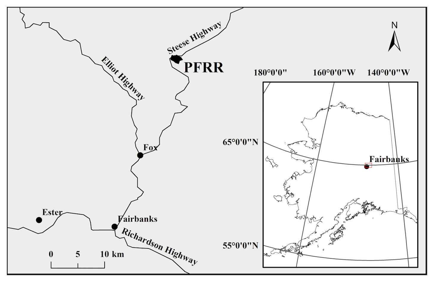
Figure 1Location of the DTS system installed at the Poker Flat Research Range (PFRR; University of Alaska Fairbanks).
The Poker Flat Research Range ( N; W, 210 m a.s.l.) is a facility managed by the University of Alaska Fairbanks (UAF) and located in the interior of Alaska, about 50 km northeast of Fairbanks (Fig. 1). The general area is part of a discontinuous permafrost zone but the site itself is underlain by permafrost with active layer thickness of about 50 to 150 cm (Nakai et al., 2013). The research site includes an observation tower built in 2010 as part of a collaboration (known as JICS) between the Japan Agency for Marine-Earth Science and Technology (JAMSTEC) and UAF's International Arctic Research Center (IARC) (Sugiura et al., 2011; Nakai et al., 2013; Ikawa et al., 2015; Nagano et al., 2018). This observation tower was used for making discrete measurements of air temperatures at 1.5 m height, short-wave radiation measurements at 16 m height (tower top), and snow depth using an ultrasonic sensor. The data from these sources were integrated into 30 min intervals prior to analysis. Measurements were conducted for a period of 2 years, from 13 October 2012 to 13 October 2014.
A ∼2.7 km fibre-optic cable was installed at the site (indicated by black line in Fig. 2a). The line traversed an irregular 2 km long path and included five different stations (numbered 1–5) with vertical temperature sensing equipment (see Sect. 2.2). The site's dominant vegetation type is black spruce, but locally the site exhibits considerable variation in surface conditions and vegetation types (see Fig. 2a). We classified land cover into six descriptive categories by applying a supervised classification algorithm (Maximum Likelihood) to RGB aerial imagery, collected on 4 September 2012. Land cover designations include relict thermokarst, lake or bare ground, open moss, shrub, deciduous forest, sparse conifer forest, and dense conifer forest. The Majority Filter tool (ArcGIS 10.3) was applied to reduce effects of speckle noise prior to classification. Figure 2b shows the occurrence frequencies of the six land cover types along the length of the cable.
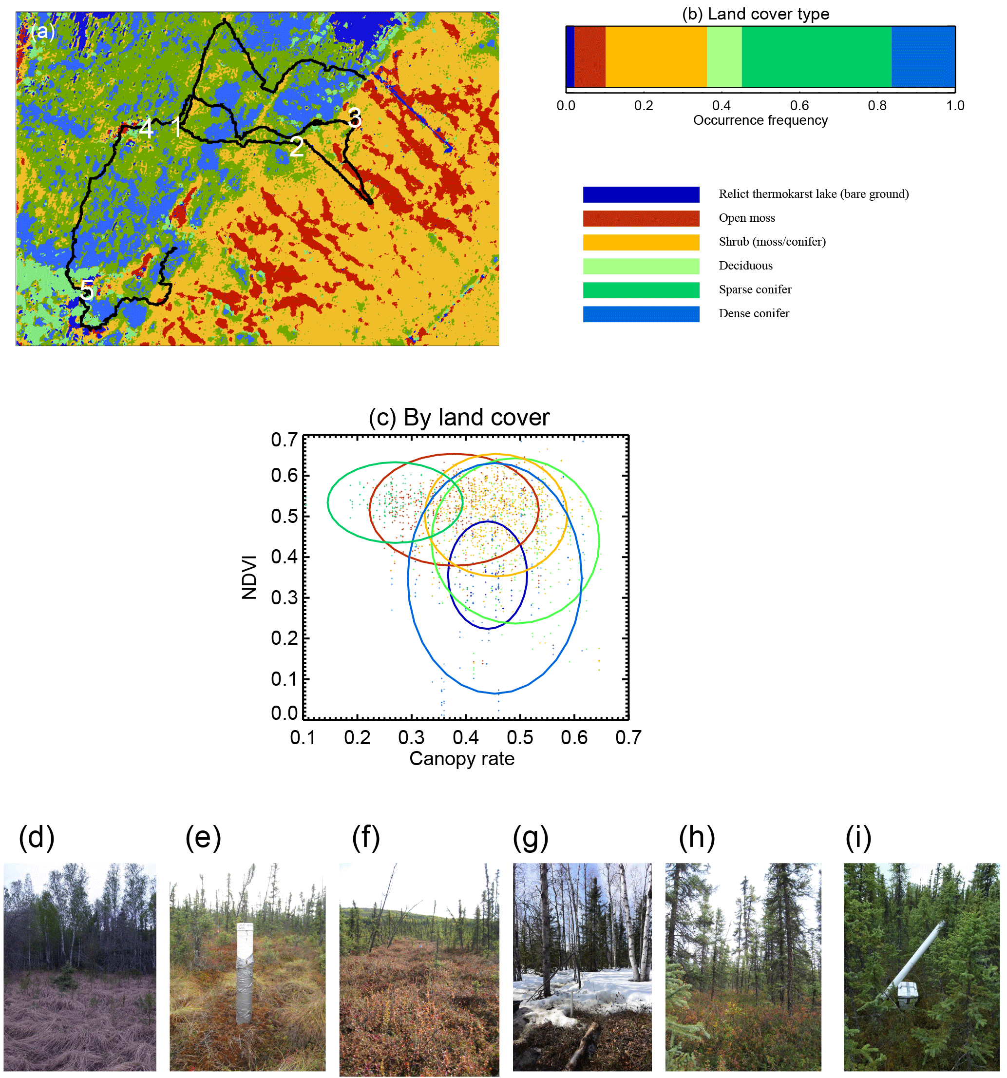
Figure 2(a) Layout of the fibre-optic cable sensor (black line) installed at the PFRR with stations numbered from 1 to 5 (in white), together with the land cover types designated from satellite images (dark blue: relict thermokarst lake, red: open moss, orange: shrubs, light green: deciduous forest, green: sparse conifer forest, blue: dense conifer forest). (b) Frequency of land cover types along the cable. (c) Scatter plot of surface-measured canopy rate and satellite-derived normalized difference vegetation index (NDVI; GeoEye1 image taken on 25 September 2010). Images show examples of (d) relict thermokarst lake, (e) open moss, (f) shrub, (g) deciduous forest, (h) sparse conifer forest, and (i) dense conifer forest.
Figure 2c shows land cover type associations along with radiative and structural canopy characteristics for each measurement segment (∼50 cm intervals) along the cable. The Normalized Difference Vegetation Index (NDVI) was derived from a GeoEye1 image taken on 25 September 2010. The canopy rate, the upper sight ratio covered by vegetation canopy when projected on a hemisphere, was calculated from a series of semi-spherical pictures taken at a height of 30 cm for every 70 cm along the cable by a THETA fish-eye camera (RICOH, Inc. cylindrical projection). Ellipses are colour-coded for each land cover type and drawn with radii representing the standard deviation in canopy rate (horizontal) and NDVI (vertical).
Figure 2d–i show typical ambient conditions for each land cover type. Relict thermokarst lake areas (Fig. 2d) include grassy depressions or flats once occupied by lakes formed by subsidence due to melting of ground ice from permafrost. This category also includes easily discernible bare grounds cleared by human activity. Open moss areas (Fig. 2e) consist of open spaces covered by moss (mainly sphagnum moss, Sphagnum fuscum, and feather moss, Hylocomium splendens) or lichens, where trees are absent. Shrub areas (Fig. 2f) are covered by dwarf to tall species. Deciduous forest land cover (Fig. 2g) consists of mixed forests with deciduous (birch, aspen, willow, etc.) and conifer (black spruce, Picea mariana, and white spruce, Picea glauca) species. The sparse conifer (Fig. 2h) and dense conifer (Fig. 2i) forest land cover types are occupied by spruces of varying density. The forest floors are mainly covered by moss with occasional shrubs where trees are sparse.
2.2 Methods
The fibre-optic DTS system deployed in this study makes use of Raman-scattering, optical time domain reflectometry techniques in measuring temperatures along the cable (Dakin et al., 1985). A laser pulse within the optical fibre (SiO2) generates back scatter radiation at different frequencies (Raman scattering). The system can record intensity ratios within the scatter spectrum (i.e. Stokes and anti-Stokes peaks). The latter peak is sensitive to the temperature of the medium. The location of the temperature measurement is derived from the travel time data (i.e. optical time domain reflectometry).
This study used a 2.7 km long fibre-optic cable (multi-mode, GI50/125, dual core; 3.4 mm, S2002A, manufactured by BRUGG, Switzerland) installed over a 2.0 km surface path (referred to as the horizontal section). Schematic illustrations of the instrument layout and experimental setup are shown in Fig. 3. Temperatures were measured at 50 cm intervals along horizontal (non-coiled) sections of the cable. Portions of the cable were also coiled around PVC tubes (effective outer diameter of 11.5 cm, and length of about 120 cm). The tubes were vertically embedded in the ground to half of their length (60 cm deep), at five stations numbered 1–5 (Fig. 2a) along the horizontal pathway. Figure 2i shows a tube prior to its installation while Fig. 2e shows a tube after installation. One loop of the coil measured about 36 cm so that three loops (ca. 1 m) corresponded to two measurement segments (each with length of 50 cm). This gave an effective vertical resolution of about 5 mm. Temperature data from the embedded tubes are referred to as vertical sections.
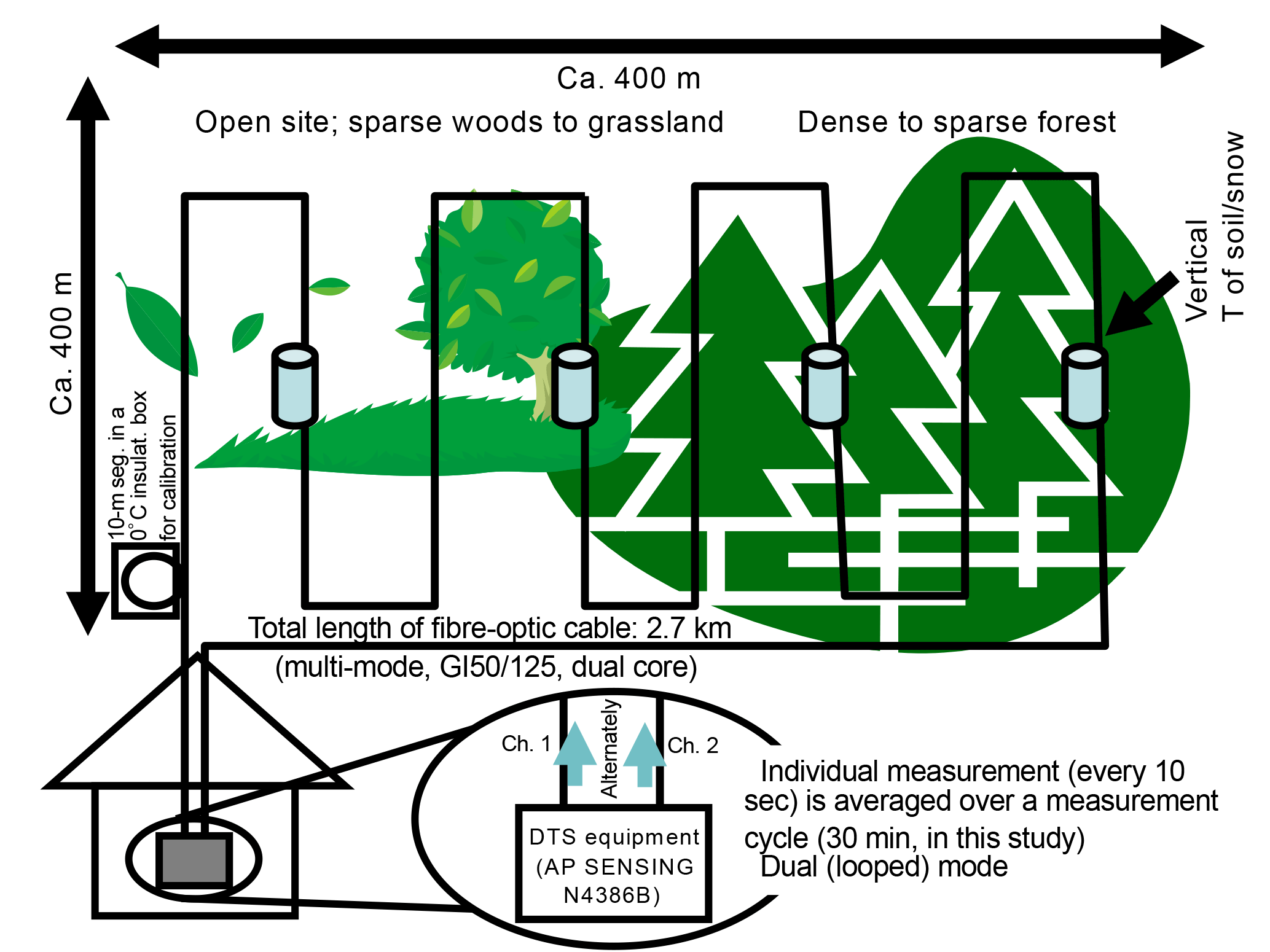
Measurements were performed in dual (looped) mode wherein the laser pulse is emitted from alternate channels at each end of the cable. Calibration was performed at 0 ∘C using a 10 m segment of the cable. The segment was coiled and kept in an insulated box filled with well mixed crashed ice and water during the calibration process for about 2 h.
Data acquired every 10 s were integrated over 30 min intervals to reduce undesirable effects of measurement error and noise. The experiment operated continuously over a 2-year interval from October 2012 to October 2014, except for several short-period disruptions due to cable or power supply failure. Temporal monitoring was referenced to Alaskan Standard Time (AKST; UTC − 9 h) and all times in this paper follow that time zone.
Figure 4 shows an example of the temperature data acquired on 1 December 2013, along a horizontal section. Figure 4a and b show the logarithmic ratio r between the anti-Stokes and Stokes components of the spectrum, and the interpreted temperature T of an instantaneous measurement made at 02:32 LT (local time or AKST, blue) and 13:39 (red). Figure 4c illustrate the respective scatter between r and T. An average over a 24 h period is shown in Fig. 4d. The daily average tower air temperature (measured at height of 1.5 m) was −32.5 ∘C and daily mean snow depth was 23.5 cm. In Fig. 4d, downward spikes correspond to temperatures of those parts of the cable exposed above the upper surface of the snow pack (minimum temperature was −32.6 ∘C while the maximum temperature was +1.0 ∘C). The temperature difference of more than 30 ∘C is likely due to combinations of the thermal effects of insulation by snow pack and of the saturation and unfrozen moisture content of the near-surface soils.
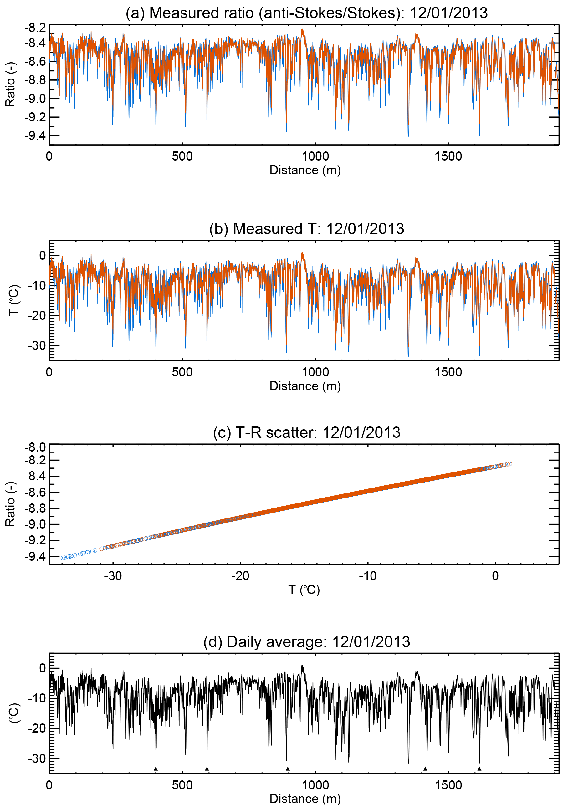
Figure 4Examples of outputs from the DTS equipment. (a) The logarithmic ratio between the Stokes and anti-Stokes components and (b) temperature of an instantaneous measurement, made at 02:32 (blue) and 13:39 (orange) on 1 December 2013, for a horizontal section of the DTS system. (c) Scatter plot between (a) and (b) for the respective time. (d) Average of the temperature measurements for the day.
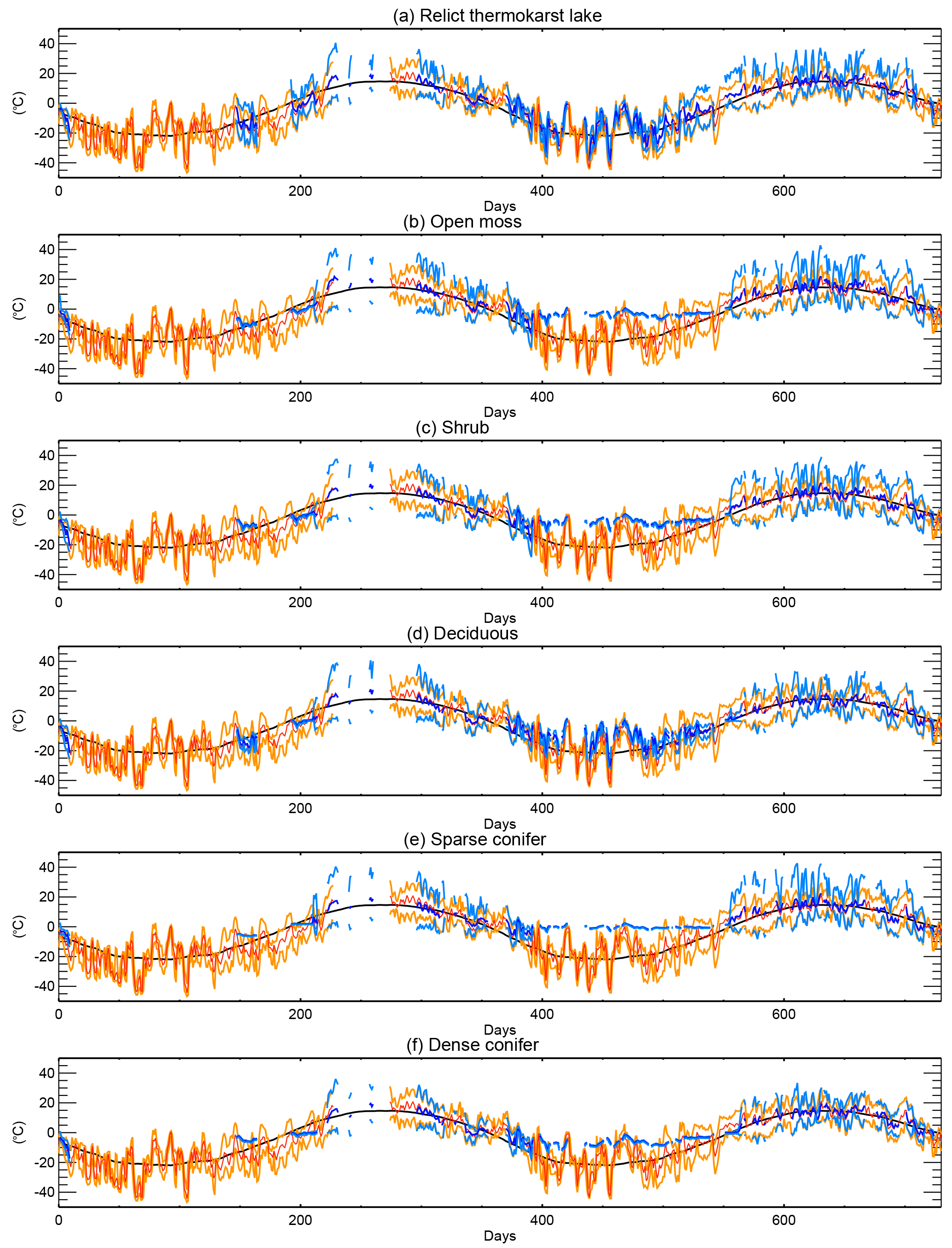
Figure 5Typical seasonal variations in daily temperatures for the six land cover types: (a) relict thermokarst lake, (b) open moss, (c) shrub, (d) deciduous forest, (e) sparse conifer forest, and (f) dense conifer forest. Plot shows daily maximum and minimum temperatures from the DTS system (blue lines) and the JICS tower (air column at 1.5 m height; orange lines) along with daily mean values (dark blue for DTS and red for the JICS tower). The black line shows daily climatology. Data span time period after 13 October 2012.
3.1 Diurnal and seasonal variation
Figure 5 shows results of DTS measurements for the six different land cover types, carried out over the 2-year period. Diurnal and seasonal variations in surface temperatures indicate the influence of both microclimates and micro-environments. Land cover types co-vary with surface conditions, canopy structure, and temporal patterns at each location. In this figure, the curves in blue colour indicate daily maximum and minimum temperatures, while the curve in dark blue colour indicates daily average temperatures. The curves in orange and red colours refer to air temperatures acquired at the JICS tower (1.5 m high). The climatological daily mean temperature is overlaid in black. The blank periods (e.g. days 10–146, 165–191, and 261–295) refer to intervals for which either DTS or tower datasets are missing. At the beginning of the 2012–2013 winter, the cable was accidentally severed at a point close to the DTS equipment. This event interrupted data collection along most of the cable section until it could be spliced back together, after the snow melt.
For the winter period (days 400–550), open moss (Fig. 5b; canopy rate = 0.29, NDVI = 0.592), shrub (Fig. 5c; canopy rate = 0.34, NDVI = 0.515), and both conifer forest types (sparse conifer in Fig. 5e; canopy rate = 0.35, NDVI = 0.531, and dense conifer in Fig. 5f; canopy rate = 0.43, NDVI = 0.495) show relatively minor variations in diurnal and daily temperatures. By contrast, thermokarst lake (Fig. 5a; canopy rate = 0.46, NDVI = 0.404) and deciduous forest (Fig. 5d; canopy rate = 0.43, NDVI = 0.239) land cover types show greater variability in daily temperatures and resume pronounced diurnal cycles relatively early on, after day 480. The ground cover for the latter two cases includes grass or limited floor vegetation, both of which are of lesser surface roughness (Fig. 2d and g). Differences between the two groups stem primarily from differences in snow pack characteristics. Snow pack tends to be thinner and effectively redistributed or blown by wind for the latter land cover types. Grasses are also prone to form void space between snow pack and the ground surface. Snow pack variation is further described in Sect. 3.2 below.
In summer time (days 220 to 350, and 570 to 700), dense conifer forest exhibited daily surface temperature ranges (DTS data) less than those observed for the air column (tower observations). By contrast, open moss, shrub, and sparse forest types showed daily surface temperature ranges that were greater than those of the overlying air column. The grassy relict lake and deciduous forest land cover types showed an intermediate response. These tendencies likely reflect the openness of the canopy (or vegetation) cover above the land surface (i.e. how much solar and long-wave radiation reach the sensor cable), as well as local albedo of different surfaces (i.e. how much the ground surface of different land cover types reflects back). Figure 6a–c show daily values (i.e. maximum, minimum, and average) for the DTS anomaly relative to the corresponding tower values for days without snow cover. Results were aggregated into four groups based on daily cloudiness, as defined by the percentage of daily total downward solar radiation between the tower (at 16 m height) and the top of the atmosphere. A box-and-whisker plot shows maximum values (100th percentile) as the top of the upper error bar, 75th percentile as the upper edge of the box, 50th percentile as the colour-coded bar, 25th percentile as the lower edge of the box, and the minimum (0th percentile) as the bottom of the lower error bar. The plot shows uniform, gradual changes in anomaly distributions from sunny days to cloudy days (Fig. 6a–c). The size of anomaly dispersions for each land cover type (represented by the total span of the whiskers) decreases with increasing cloud cover, due to cloud diffusing effects. Daily average temperatures at the surface generally exceed those observed by the JICS tower (at 1.5 m height). Daily maximum values appear to contribute to this effect more than daily minimum values do. The latter (daily minimum) values are closer to the tower-observed values. Among different land cover types, open moss and deciduous forest tend to give higher daily maximum and lower daily minimum anomalies.

Figure 6Distributional differences between (a) daily maximum temperatures, (b) daily minimum temperatures, and (c) daily average temperature under different degrees of cloudiness (32 observations for 0–25 %, 69 observations for 25–50 %, 80 observations for 50–75 %, and 5 observations for 75–100 %). Lower plots show median maximum (d) and minimum (e) temperature values and frequency (total hours) as measured by DTS for land cover types (colour-coded) compared to corresponding values from the JICS tower (1.5 m height; black-line histogram).
Figure 6d and e show phases of diurnal extremes (i.e. exact time of either the original daily maximum or daily minimum temperature) for the DTS (colour-coded bars) and JICS tower (black line) observations, respectively. The daily maximum for surface temperatures (Fig. 6d) are reached 2 h before that of the air temperature. Relict thermokarst lake areas (grassy or bare grounds) tend to reach the daily maximum temperature earlier and deciduous forest areas later than other land cover types. For the daily minimum temperature (Fig. 6e), surface and air temperatures are more in-phase with each other. This temperature is reached in the 3rd to 4th hour (03:00–04:00 LT) slot for a normal daily cycle, or at the 23rd to 24th hour (23:00–00:00 LT).
3.2 Spatial snow cover characteristics
As shown in Fig. 5, snow pack greatly affects wintertime thermal conditions at the interface between the ground and snow pack. Snow cover on the ground surface strongly influences the radiative and energy budget, the water cycle, and phenology (Sturm et al., 2005; Liston, 1999; Tan et al., 2011; Immerzeel et al., 2010; Jönsson et al., 2010). Seasonal snow pack data (e.g. timing of when/how snow pack accumulates and disappears) is important for interpreting observed temperature values and for constraining energy budgets within numerical models. Snow pack is affected by the land cover types, which can amplify contrasting conditions (Liston, 1999, 2004; Sturm et al., 2005). Here, we describe how DTS data indicate different trajectories of snow pack evolution (namely appearance and disappearance) and produce apparent insulation effects for different land cover types.
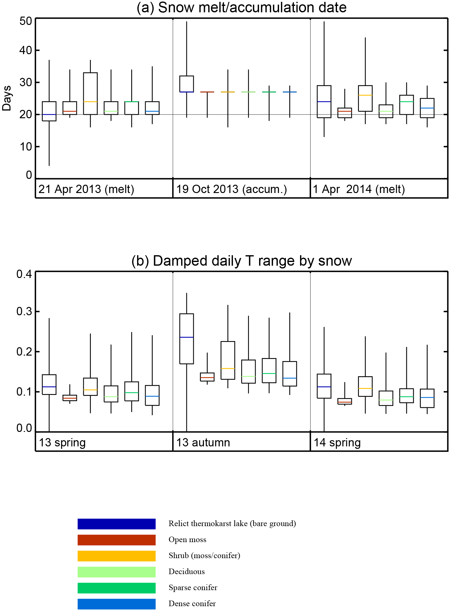
Figure 7(a) Differences in snow melt (or accumulation) dates for different land cover types for the spring of 2013 (after 21 April 2013), autumn of 2013 (after 19 October 2013), and spring of 2014 (after 1 April 2014). (b) Damping rate for daily temperature range averaged over snow-covered days having continuous measurements (i.e. without missing or interrupted cable data) for the 50-day period following the respective start date of the season.
Figure 7a shows dates of initial snow accumulation (the middle panel) and final disappearance (left and rightmost panels) for each land cover type, as counted from the date shown at the bottom of the respective panel. The presence of a continuous snow cover was defined considering the periods during which the daily amplitude in DTS temperatures fell short of 40 % of that of the JICS tower (1.5 m high) observations. As shown in Fig. 7b, this 40 % threshold effectively differentiates between snow-free and snow-covered conditions. The overall contrast between accumulation and disappearance dates (Fig. 7a) indicates that accumulation of snow cover tends to begin as spatially coherent and widespread, whereas disappearance of snow pack varies according to local conditions (Liston, 2004; Nitta et al., 2014). Among different land cover types, the majority (denoted by the margin between the 25th percentile and 75th percentile) of grassy (relict thermokarst lakes; blue) and shrubby (shrub; orange) areas vary more widely than the forest land cover types do (greens). Open moss (red) of relatively flat areas shows equal or greater variation than forest land cover types.
Another important geophysical effect of snow cover is the insulation it provides between the atmosphere and land surface. Figure 7b demonstrates this effect by showing the reduction in daily temperature range for the ground surface relative to the air. Open moss land cover shows the most spatially coherent and pronounced reduction. This implies spatial homogeneity in snow pack depth and physical properties (e.g. density, shape and size of snow grain, snow class), which could contribute to similar timing of snow disappearance (Fig. 7a). The strong insulation effect likely results from development of the depth hoar layer by radiative cooling. Relict thermokarst lake areas show high spatial variability in temperature range reduction. Forested land cover showed small reductions regardless of the vegetation types, possibly due to cooler ambient conditions beneath the canopy.
3.3 Vertical temperature profiles
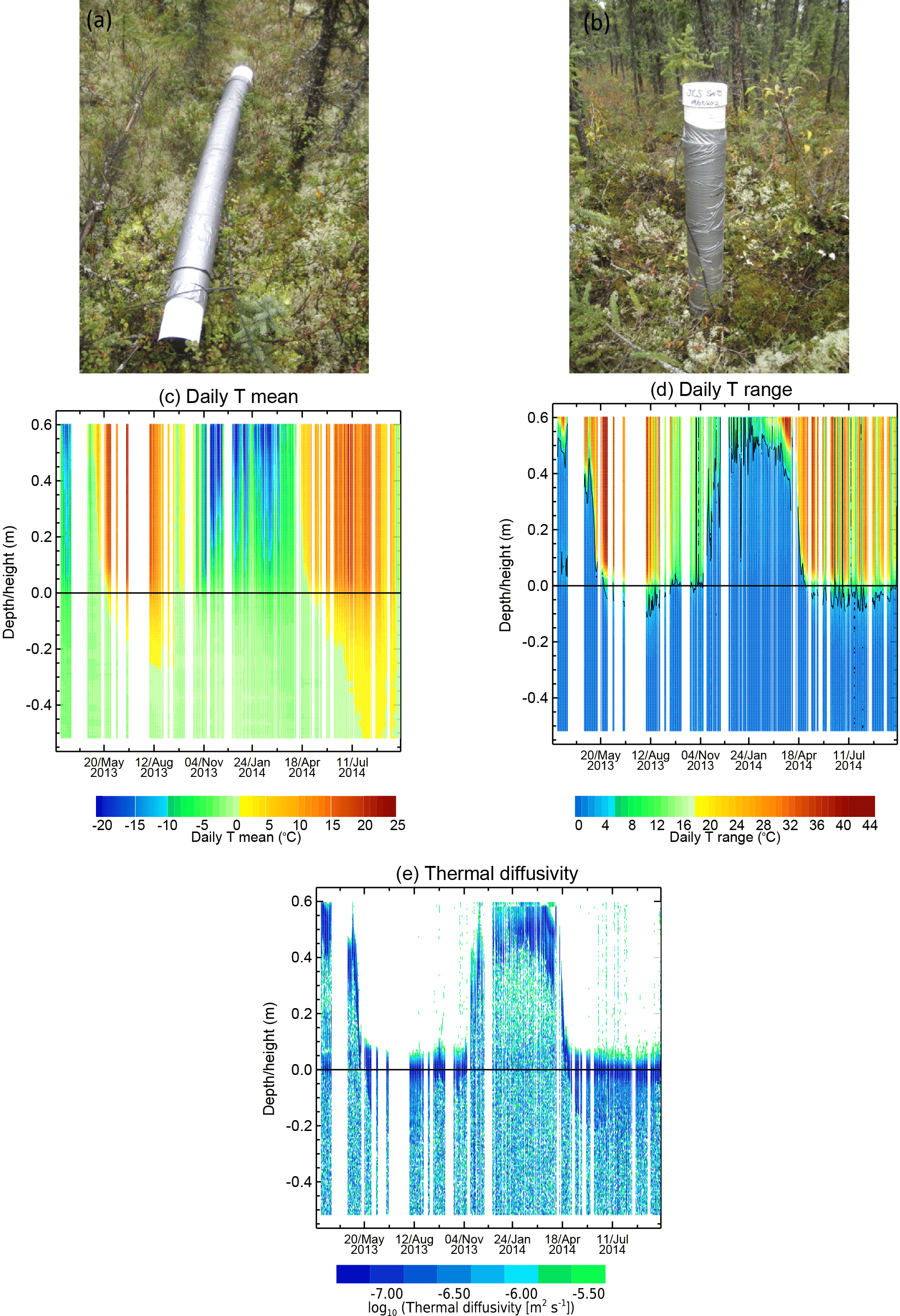
Figure 8Subsurface and above-surface temperatures measured by vertical sections. (a) Photo of PVC tube with sensor cable wrapping prior to installation. (b) Photo of PVC tube with temperature sensor (vertical section) installed within a dense conifer forest. Depth-time profiles for (c) daily mean temperatures and (d) daily temperature range during 2013 snow melt period. (e) Same as (c) except for apparent thermal diffusivity (m2 s−1), shown in common logarithmic scale.
The fibre-optic cable wrapped around a 120 cm long PVC tube (Fig. 8a–b) provided high-resolution vertical temperature profiles for ground, air, and snow columns at five stations each situated within different land cover types (Fig. 2a).
Station no. 1 is located in dense forest, no. 2 in sparse forest, no. 3 in open moss, no. 4 in shrub, and no. 5 in a relict thermokarst lake area. Figure 8c–d show seasonal changes in daily mean temperature and temperature range, respectively, for station no. 1. White areas represent missing values due to either cable disruption or other technical issues. Blue areas in Fig. 8d show daily temperature values whose ranges are curtailed either by snowpack (above ground for the part above the black line) or ground (below the black line). Together with Fig. 8c, d shows the different characteristics in temperature variations between the air, and snow pack above the ground, and between frozen or thawed periods below the surface. One of the geophysical applications of the vertical profile data is calculation of apparent thermal diffusivity. The general analytical solution of the transient conduction heat transfer equation (cf. Horton et al., 1983) is
where T is temperature and α is thermal diffusivity (m2 s−1), with a diurnal sinusoidal boundary condition, and can be used to derive the ratio of the daily amplitude r between two layers of distance D as
where ω is the frequency for a day. Applying Eq. (2) to the daily temperature range data (e.g. Fig. 8d) yields the distribution of the apparent thermal diffusivity (Fig. 8e; shown in common logarithmic scale). Since it includes effects of nonconductive heat transfer such as latent heat (phase change) and convective heat transfer, it is different from true thermal diffusivity. It should also be noted that the observed diurnal cycle is not always sinusoidal. However, the calculated values clearly depict the areas of melting of snow and thawing of soil with decreased values (because of an increase in apparent heat capacity due to phase change), which are smaller than the typical true thermal diffusivity values for ice (roughly, m2 s−1 at −1∘; its common logarithm is −5.94) and water (similarly, m2 s−1 at 0∘, with its common logarithm −6.85). The front line of thawing soil (appeared after snow melt in both years) is evidently shown down to the depth of 20 to 25 cm, below which the attenuated diurnal component in conductive heat transfer are effectively damped.
As described above, DTS provides continuous records suitable for analysis of spatial variability in temperature. Data acquisition, however, depends on uninterrupted functioning of fibre-optic cables and uninterrupted power and communication capabilities, which in turn depend on robust equipment performance under harsh and highly variable local climate conditions. This section describes specific technical and environmental challenges identified during our study.
A continuous electrical power supply is critical for remote DTS field data collection. This requirement limits locations where DTS apparatus can be deployed. Even when available, the power system used here was subject to harsh temperature and precipitation conditions. A durable, uninterrupted power supply (a.k.a. UPS) is recommended for future experiments. Fibre-optic cables also pose significant logistical challenges when deployed in remote taiga forest environments. Irregular surface areas with variable moisture and numerous obstacles (such as trees) prevent construction of a simple, protected route for the cable. Deploying a ∼3 km long cable from a large wooden spool, which together with the cable weighed more than 50 kg, around barriers and across soggy ground posed significant challenges. We chose a cable with a stainless-steel shielding tube to optimize sensing capabilities but also to protect against disruption by animals. The shielding turned out to have suboptimal flexibility (compared to that of woven stainless mesh shielding), which led to kinking and even breaking during installation. The tube-shielded cable was also too inflexible for the irregular ground surface.
A better approach for cable routing would be to use a smaller, lighter spool and shorter cable, installing the sensor as a series of shorter cable segments. A fusion splicer, already necessary for cable repair, could be used to splice shorter segments of cable in the field instead of installation of a single long cable. Cable splicing and repair requires some training and experience, especially for performing correct core alignment under field conditions. Splicing is also not possible under harsh winter conditions (e.g. −20 ∘C or below), even though the cable and DTS still function at these temperatures.
The DTS system is also vulnerable to cable breaks. Once the cable breaks, it cannot measure temperature beyond that point. For example, if the cable breaks at 1 m of a 1 km cable system, the remaining 999 m will produce no data. Dual-mode measurement (a cable loop connected to two channels at both ends) can prevent total loss of measurements beyond the break, although the resulting single-mode measurements need additional calibration.
We deployed a fibre-optic DTS (distributed temperature sensing) system, which uses techniques of optical time domain reflectometry to measure spatial and temporal variation in surface temperatures of a northern forest (taiga) site situated in the interior of Alaska. The DTS system consists of a 2.7 km fibre-optic cable, sections of which are installed on, above, and below surface areas with a range of different land cover types. The system provided continuous temperature data at half-metre distance intervals and 30 min time periods. The site, the Poker Flat Research Range (managed by the University of Alaska Fairbanks), is underlain by permafrost and primarily covered by black spruce. Land cover types of the study area include relict thermokarst lake, open moss, shrub, deciduous forest, sparse conifer forest, and dense conifer forest. The DTS system collected data over a 2-year period, from October 2012 to October 2014.
Data from horizontal sections of the DTS system (about 2.0 km of the cable) recorded diurnal and seasonal temperature variations occurring in different land cover types and surface conditions. Snow and canopy effects, for example, were evident in spatiotemporal temperature patterns. Data from vertical sections (cable wrapped around PVC tubes embedded in the ground) recorded air, snow, and ground temperatures at high resolution (∼5 mm).
The DTS system proved operable and useful for geophysical investigations in the harsh taiga environment, which experiences annual temperature ranges of −40 to 30 ∘C. However, the system also faced technical challenges in attempting continuous temperature measurements of the local environment. Future activities will continue to optimize DTS systems for geoscientific research in taiga areas and other similar environments.
The DTS measurement data analysed in this paper along with supplementary information are archived and accessible at the International Arctic Research Center (IARC) data archive of the University of Alaska Fairbanks (http://climate.iarc.uaf.edu/geonetwork/srv/en/main.home?uuid=60804e98-a0d5-4bcc-ab70-5d47af2b50ca, Saito, 2018).
KS designed and prepared the experiment. All authors took part in the tasks of deployment of the equipment and maintenance of the measurement system. KS prepared the manuscript with contributions from all coauthors.
The authors declare that they have no conflict of interest.
This study was conducted as a part of JAMSTEC-IARC Collaboration Study
(JICS). This work was partially supported by the Program for Risk Information
on Climate Change (SOUSEI program), the Integrated Research Program for
Advancing Climate Models (TOUGOU program), and the Arctic Challenge for
Sustainability (ArCS) program, the Japanese Ministry of Education, Culture,
Sports, Science, and Technology, and by the Environmental Research and
Technology Development Fund 2-1605 of the Japanese Ministry of Environment
and Environmental Restoration and Conservation Agency. The Poker Flat
Research Range kindly provided the facility and necessary logistics for the
installments and the measurement operations. Authors gratefully acknowledge
assistance from Kyotaro Noguchi, Ryouta O'ishi, Shinji Matsumura, Taro Nakai, Yasunori Igarashi, and Larsen Hess for installing the fibre-optic cables at the PFRR site, and
NK Systems Limited for advice and guidance on the DTS settings and
operations.
Edited by: Lev Eppelbaum
Reviewed by: two anonymous referees
Beer, C., Lucht, W., Gerten, D., Thonicke, K., and Schmullius, C.: Effects of soil freezing and thawing on vegetation carbon density in Siberia: a modeling analysis with the Lund–Potsdam–Jena dynamic global vegetation model (LPJ-DGVM), Global Biogeochem. Cy., 21, GB1012, https://doi.org/10.1029/2006GB002760, 2007.
Dakin, J. P., Pratt, D. J., Bibby, G. W., and Ross, J. N.: Raman temperature sensor using a semiconductor light source and detector, Electron. Lett., 21, 569–570, 1985.
Dyer, S. D., Tanner, M. G., Baek, B., Hadfield, R. H., and Nam, S. W.: Analysis of a distributed fiber-optic temperature sensor using single-photon detectors, Opt. Express, 20, 3456–3466, 2012.
Essery, R. L. H., Rutter, N., Pomeroy, J., Baxter, R., Staehli, M., Gustafsson, D., Barr, A., Bartlett, P., and Elder, K.: SnowMIP2: An evaluation of forest snow process simulations, B. Am. Meteorol. Soc., 90, 1120–1135, https://doi.org/10.1175/2009BAMS2629.1, 2009.
Euskirchen, E. S., McGuire, A. D., Kicklighter, D. W., Zhuanf, Q., Clein, J. S., Dargaville, R. J., Dye, D. G., Kimball, J. S., McDonald, K. C., Melillo, J. M., Romanovsky, V. E., and Smith, N. V.: Importance of recent shifts in soil thermal dynamics on growing season length, productivity, and carbon sequestration in terrestrial high-latitude ecosystems, Glob. Change Biol., 12, 731–750, 2006.
Horton, R., Wierenga, P. J., and Nielsen, D. R.: Evaluation of methods for determining the apparent thermal diffusivity of soil near the soil surface, Soil Sci. Soc. Am. J., 47, 25–32, 1983.
Ikawa, H., Nakai, T., Busey, R. C., Kim, Y., Kobayashi, H., Nagai, S., Ueyama, M., Saito, K., Nagano, H., Suzuki, R., and Hinzman, L.: Understory CO2, sensible heat, and latent heat fluxes in a black spruce forest in interior Alaska, Agr. Forest Meteorol., 214–215, 80–90, 2015.
Immerzeel, W. W., van Beek, L. P. H., and Bierkens, M. F. P.: Climate change will affect the Asian water towers, Science, 328, 1382–1385, https://doi.org/10.1126/science.1183188, 2010.
IPCC: Climate Change 2013: The Physical Science Basis, Contribution of Working Group I to the Fifth Assessment Report of the Intergovernmental Panel on Climate Change, edited by: Stocker, T. F., Qin, D., Plattner, G.-K., Tignor, M., Allen, S. K., Boschung, J., Nauels, A., Xia, Y., Bex, V., and Midgley, P. M., Cambridge University Press, Cambridge, UK and New York, NY, USA, 1535 pp., 2013.
Jönsson, A. M., Eklundh, L., Hellstrom, M., Barring, L., and Jonsson P.: Annual changes in MODIS vegetation indices of Swedish coniferous forests in relation to snow dynamics and tree phenology, Remote Sens. Environ., 114, 2719–2730, 2010.
Kasurinen, V., Alfresdsen, K., Kolari, P., Mammarella, I., Alekseychik, P., Rinne, J., Vesala, T., Bernier, P., Boike, J., Langer, M., Belelli Marchesini, L., Huissteden, K., Dolman, H., Sachs, T., Ohta, T., Varlagin, A., Rocha, A., Arain, A., Oechel, W., Lund, M., Grelle, A., Lindroth, A., Black, A., Aurela, M., Laurila, T., Lohila A., and Beringer, F.: Latent heat exchange in the boreal and arctic biomes, Glob. Change Biol., 20, 3439–3456, https://doi.org/10.1111/gcb.12640, 2014.
Liston, G. E.: Interrelationships among Snow Distribution, Snowmelt, and Snow Cover Depletion: Implications for Atmospheric, Hydrologic, and Ecologic Modeling, J. Appl. Meteorol., 38, 1474–1487, 1999.
Liston, G. E.: Representing sub-grid snow cover heterogeneities in regional and global models, J. Climate, 17, 1381–1397, https://doi.org/10.1175/1520-0442(2004)017<1381:RSSCHI>2.0.CO;2, 2004.
Lutz, J. A., Martin, K. A., and Lundquist, J. D.: Using Fiber-Optic Distributed Temperature Sensing to Measure Ground Surface Temperature in Thinned and Unthinned Forests, Northwest Sci., 86, 108–121, https://doi.org/10.3955/046.086.0203, 2012.
Nagano, H., Ikawa, H., Nakai, T., Matsushima-Yashima, M., Kobayashi, H., Kim, Y., and Suzuki, R.: Extremely dry environment down-regulates nighttime respiration of a black spruce forest in Interior Alaska, Agr. Forest Meteorol., 249, 297–309, https://doi.org/10.1016/j.agrformet.2017.11.001, 2018.
Nakai, T., Kim, Y., Busey, R. C., Suzuki, R., Nagai, S., Kobayashi, H., Park, H., Sugiura, K., and Ito, A.: Characteristics of evapotranspiration from a permafrost black spruce forest in interior Alaska, Polar Sci., 7, 136–148, 2013.
Nitta, T., Yoshimura, K., Takata, K., Oíshi, R., Sueyoshi, T., Kanae, S., Oki, T., Abe-Ouchi, A., and Liston, G. E.: Representing Variability in Subgrid Snow Cover and Snow Depth in a Global Land Model: Offline Validation, J. Climate, 27, 3318–3330, https://doi.org/10.1175/JCLI-D-13-00310.1, 2014.
Ohta, T., Maximov, T. C., Dolman, A. J., Nakai, T., van der Molen, M. K., Kononov, A. V., Maximov, A. P., Hiyama, T., Iijima, Y., Moors, E. J., Tanaka, H., Toba, T., and Yabuki, H.: Interannual variation of water balance and summer evapotranspiration in an eastern Siberian larch forest over a 7-year period (1998–2006), Agr. Forest Meteorol., 148, 1941–1953, 2008.
Piao, S. L., Ciais, P., Friedlingstein, P., Peylin, P., Reichstein, M., Luyssaert, S., Margolis, H., Fang, J. Y., Barr, A., Chen, A. P., Grelle, A., Hollinger, D. Y., Laurila, T., Lindroth, A., Richardson, A. D., and Vesala, T.: Net carbon dioxide losses of northern ecosystems in response to autumn warming, Nature, 451, 49-U43, https://doi.org/10.1038/nature06444, 2008.
Pomeroy, J., Rowlands, A., Hardy, J., Link, T., Marks, D., Essery, R., Sicart, J. E., and Ellis, C.: Spatial Variability of Shortwave Irradiance for Snowmelt in Forests, J. Hydrometeorol., 9, 1482–1490, https://doi.org/10.1175/2008JHM867.1, 2008.
Purdy, A. J., Fisher, J. B., Goulden, M. L., and Famiglietti, J. S.: Ground heat flux: an analytical review of 6 models evaluated at 88 sites and globally, J. Geophys. Res.-Biogeo., 121, 3045–3059, https://doi.org/10.1002/2016JG003591, 2016.
Rutter, N., Essery, R., Pomeroy, J., Altimir, N., Andreadis, K., Baker, I., Barr, A., Bartlett, P., Boone, A., Deng, H., Douville, H., Dutra, E., Elder, K., Ellis, C., Feng, X., Gelfan, A., Goodbody, A., Gusev, Y., Gustafsson, D., Hellström, R., Hirabayashi, Y., Hirota, T., Jonas, T., Koren, V., Kuragina, A., Lettenmaier, D., Li, W. P., Luce, C., Martin, E., Nasonova, O., Pumpanen, J., Pyles, R. D., Samuelsson, P., Sandells, M., Schädler, G., Shmakin, A., Smirnova, T. G., Stähli, M., Stöckli, R., Strasser, U., Su, H., Suzuki, K., Takata, K., Tanaka, K., Thompson, E., Vesala, T., Viterbo, P., Wiltshire, A., Xia, K., Xue, Y., and Yamazaki, T.: Evaluation of forest snow processes models (SnowMIP2), J. Geophys. Res., 114, D06111, https://doi.org/10.1029/2008JD011063, 2009.
Saito, K.: Fibre-optic distributed temperature monitoring (DTS) system at a boreal forest PFRR site: Loop 1, available at: http://climate.iarc.uaf.edu/geonetwork/srv/en/main.home?uuid=60804e98-a0d5-4bcc-ab70-5d47af2b50ca, last access: 26 July 2018.
Sato, H., Kobayashi, H., Iwahana, G., and Ohta, T. Endurance of larch forest ecosystems in eastern Siberia under warming trends, Ecol. Evol., 5690–5704, 2016.
Selker, J. S., van de Giesen, N., Westhoff, M., Luxemburg, W., and Parlange, M. B.: Fiber optics opens window on stream dynamics, Geophys. Res. Lett., 33, L24401, https://doi.org/10.1029/2006GL027979, 2006a.
Selker, J. S., Thévenaz, L., Huwald, H., Mallet, A., Luxemburg, W., van de Giesen, N., Stejskal, M., Zeman, J., Westhoff, M., and Parlange, M. B.: Distributed fiber-optic temperature sensing for hydrologic systems, Water Resour. Res., 42, W12202, https://doi.org/10.1029/2006WR005326, 2006b.
Sellers, P.: Modeling and observing land-surface-atmosphere interactions on large scales, Surv. Geophys., 12, 85–114, 1991.
Soto, M. A., Ramírez, J. A., and Thévenaz, L.: Intensifying the response of distributed optical fibre sensors using 2D and 3D image restoration, Nat. Commun., 7, 10870, https://doi.org/10.1038/ncomms10870, 2016.
Sugiura, K., Suzuki, R., Nakai, T., Busey, R. B., Hinzman, L. D., Park, H., Kim, Y., Nagai, S., Saito, K., Cherry, J. E., Ito, A., Ohata, T., and Walsh, J.: Supersite as a common platform for multi-observations in Alaska for a collaborative framework between JAMSTEC and IARC, JAMSTEC Rep. Res. Dev., 12, 61–69, 2011.
Sturm, M., Schimel, J., Michaelson, G., Welker, J. M., Oberbauer, S. F., Liston, G. E., Fahnestock, J., and Romanovsky, V. E.: Winter Biological Processes Could Help Convert Arctic Tundra to Shrubland, BioScience, 55, 17–26, 2005.
Tan, A., Adam, J. C., and Lettenmaier, D. P.: Change in spring snowmelt timing in Eurasian Arctic rivers. J. Geophys. Res., 116, D03101, https://doi.org/10.1029/2010JD014337, 2011.
Thomas, C. K., Kennedy, A. M., Selker, J. S., Moretti, A., Schroth, M. H., Smoot, A. R., Tufillaro, N. B., and Zeeman, M. J.: High-Resolution Fibre-Optic Temperature Sensing: A New Tool to Study the Two-Dimensional Structure of Atmospheric Surface-Layer Flow, Bound.-Lay. Meteorol., 142, 177–192, https://doi.org/10.1007/s10546-011-9672-7, 2012.
Tyler, S. W., Selker, J. S., Hausner, M. B., Hatch, C. E., Torgersen, T., Thodal, C. E., and Schladow, S. G.: Environmental temperature sensing using Raman spectra DTS fiber-optic methods, Water Resour. Res., 45, W00D23, https://doi.org/10.1029/2008WR007052, 2009.
Vrese, P., Schulz, J.-P., and Hagemann, S.: On the Representation of Heterogeneity in Land-Surface–Atmosphere Coupling, Bound.-Lay. Meteorol., 160, 157–183, 2016.