the Creative Commons Attribution 4.0 License.
the Creative Commons Attribution 4.0 License.
 | 14 Dec 2018
Mars submillimeter sensor on microsatellite: sensor feasibility study
Yasuko Kasai
Takeshi Kuroda
Shigeru Sato
Takayoshi Yamada
Hiroyuki Maezawa
Yutaka Hasegawa
Toshiyuki Nishibori
Shinichi Nakasuka
Paul Hartogh
We present a feasibility study for a submillimeter instrument on a small Mars platform now under construction. The sensor will measure the emission from atmospheric molecular oxygen, water, ozone, and hydrogen peroxide in order to retrieve their volume mixing ratios and the changes therein over time. In addition to these, the instrument will be able to limit the crustal magnetic field, and retrieve temperature and wind speed with various degrees of precision and resolution. The expected measurement precision before spatial and temporal averaging is 15 to 25 ppmv for the molecular oxygen mixing ratio, 0.2 ppmv for the gaseous water mixing ratio, 2 ppbv for the hydrogen peroxide mixing ratio, 2 ppbv for the ozone mixing ratio, 1.5 to 2.5 µT for the magnetic field strength, 1.5 to 2.5 K for the temperature profile, and 20 to 25 m s−1 for the horizontal wind speed.


We are building a submillimeter sensor intended to fly on a microsatellite platform in Mars orbit. The goal is to launch in 2024, and the main scientific target is to measure changes in Martian molecular oxygen over time. The sensor is based on a previous proposal of a more advanced version of the instrument by Kasai et al. (2012), and our working name for the sensor and platform is the Terahertz Experiment (TEREX). As both Urban et al. (2005) and Kasai et al. (2012) have previously suggested, the advantages of submillimeter technology for Martian remote sensing is that the radiation at submillimeter frequencies is mostly unaffected by atmospheric dust content, and that the radiation observed is passively emitted by the target atmospheric gases. The sensor will be able to measure molecular oxygen, gaseous water, hydrogen peroxide, ozone, the temperature field, the wind field, and the strongest crustal magnetic fields. These observations are possible from radiation emitted from within dust storms and are independent of the local time.
Martian molecular oxygen has been measured several times by missions like Viking, Herschel, Curiosity, and MAVEN. Carleton and Traub (1972) measured a global molecular oxygen profile of 1300 ppmv, Hartogh et al. (2010) measured a constant 1400 ppmv profile in whole disk measurements but remarked that there could be a higher concentration near the surface, Mahaffy et al. (2013) measured a constant profile of 1450 ppmv in ground-based measurements, and Sandel et al. (2015) measured up to 4000 ppmv at altitudes of 90 to 120 km in limb measurements at nanometer wavelengths. The discrepancies are small between most of these, but they are important and should be studied in more detail. Molecular oxygen acts as the chemical background that oxidizes gaseous water and various hydrogen radicals. Low-altitude variations have not been measured in detail over time. The Sandel et al. (2015) results shows that the profile cannot be constant from the ground up to 90 km, so the volume mixing ratio must increase over some altitude range. However, our sensor will not be able to confirm these measurements because the altitude range of Sandel et al. (2015) is above our reach. Instead, the instrument we describe here will be able to see if the increases observed at 90 km are reflected near the surface and provide a constraint on the altitude range at which the relative oxygen concentration starts increasing. Another of the key features of Mars that our sensor can help with is measuring some aspects of dust-storm-induced chemistry. Dust storms can have large electric fields, which means that there will be a large increase in hydrogen peroxide when these storms are active (Atreya et al., 2006; Delory et al., 2006). Since submillimeter waves are barely affected by atmospheric dust, the instrument will be able to sense hydrogen peroxide production inside the dust cloud.
This paper is dedicated to showing a feasibility study we performed to test the sensor design of TEREX. There will be other papers about the mission to describe the details of the orbit insertion and retention, and to give a broader scientific overview of the mission as a whole. This paper shows the forward simulations of the expected observations and the error estimations from a simple retrieval setup. The next section describes the method we used to set up our simulations – it also discusses some of the limitations that we have encountered. After the description of our method, we show our results, discuss their consequences, and give our concluding remarks.
This section goes through the basic assumptions we made to perform the simulations. This includes orbit considerations, sensor design, spectroscopic modeling, and retrieval procedure.
2.1 Orbit
The submillimeter sensor will be carried to Mars on a satellite weighing less than 100 kg. Such a small satellite needs special means to enter orbit. The selected method to achieve orbit is to use the atmospheric drag to perform aerocapture. Aerocapture has never been attempted successfully before – as far as we are aware – so the final orbital parameters are to some extent uncertain. A future work will discuss the orbit insertion and retention in details. For this work, we have opted to work simply with two sets of observations taken from an orbit with the Kepler element's semi-major axis of 6150 km and eccentricity of 0.5. This gives a periareion altitude of 400 km and an orbit time of 5 h and 20 min. We will show simulated observations as well as estimated errors for retrieved atmospheric quantities in limb-scanning mode near the periareion and in nadir-staring mode near the apoareion. The final orbit could differ from the one above, but the feasibility of the sensor is not strictly dependent on the details of the orbit. As long as the periareion is not too high, it will merely affect its spatial resolution.
2.2 Sensor
The sensor is also limited in mass and power budget by the small scale of the platform itself. We will, for instance, not be able to change the local oscillator to be sensitive to different ranges than those selected on the design board. A schematic sketch of the instrument can be seen in Fig. 1. The spectrometer we plan to use is the chirp transform spectrometer designed for the Jupiter icy moon explorer's submillimeter wave instrument, with 10 000 channels over a 1 GHz range (Hartogh, 1997; Hartogh and Hartmann, 1990; Hartogh and Osterschek, 1995; Paganini and Hartogh, 2009; Villanueva and Hartogh, 2004; Villanueva et al., 2006). The local oscillator will be at 481.15 GHz with a central intermediate frequency of 6 GHz. There will be no suppression of either of the sidebands, so the measured radiation will be between 474.65–475.65 and 486.65–487.65 GHz. The system noise temperature is expected to be about 2000 K in double-sideband mode. The antenna is planned to be 30 cm large and made of carbon fiber reinforced plastic. This achieves a 10 km vertical footprint at orbit altitudes below about 400 km, with a resolution half-width of about 0.14∘. A lower system noise would improve all results presented below, though the quoted number is as good as we expect the instrument will be at time of flight.
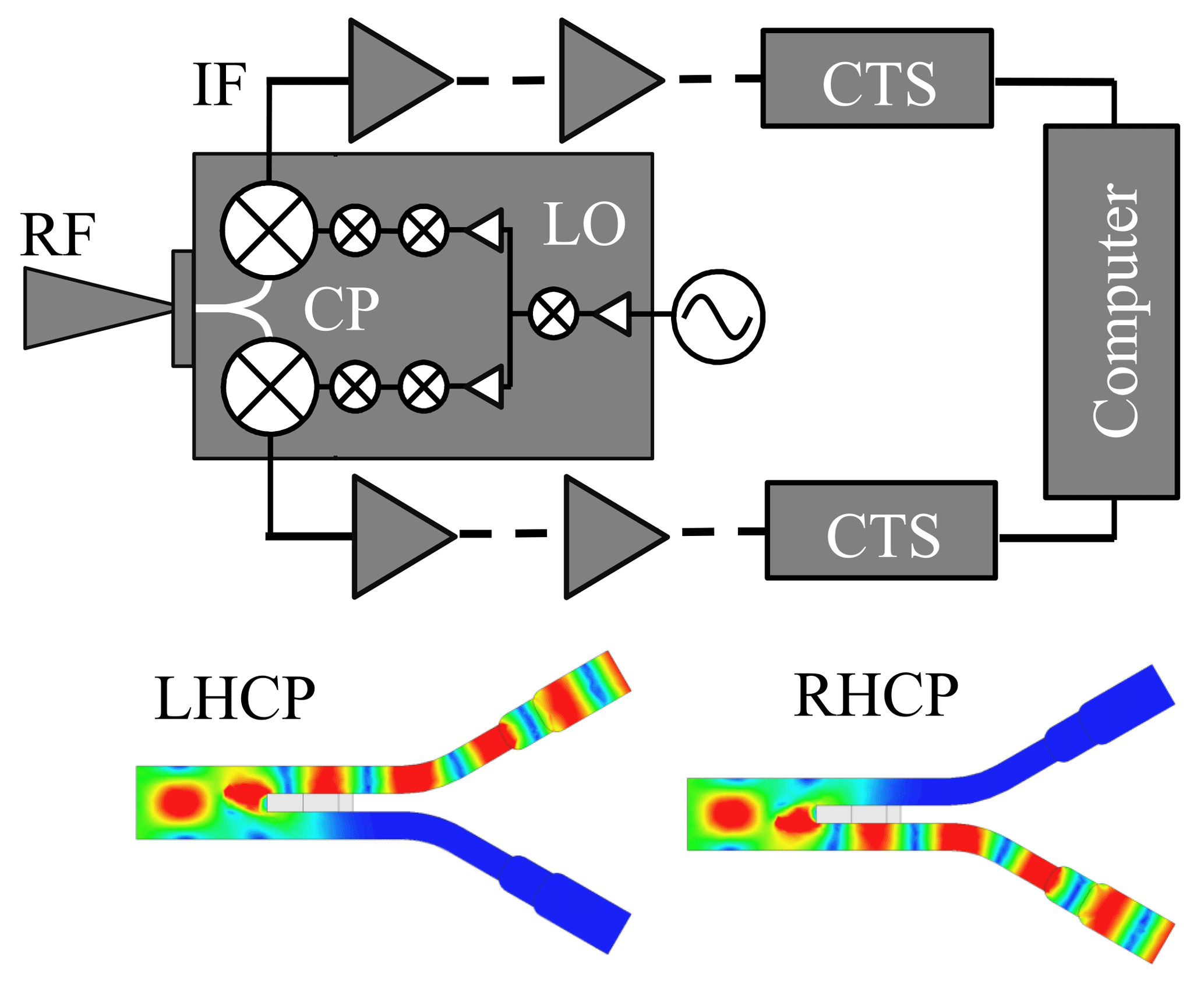
Figure 1Sketch of sensor electronics design. The radio frequency (RF) between 474.65–475.65 and 486.65–487.65 GHz enters from the left in the figure and is split by a circular polarizer (CP) into left-handed, and right-handed, circular polarization (LHCP, RHCP) as demonstrated in the colored plots above. The signal is then mixed with the signal of a local oscillator at 481.15 GHz, to lower the frequency to a measurable range. At an intermediate frequency of 6 GHz, the chirp transform spectrometer turns this analog signal into a digital signal that is fed into a computer for preparations and to be sent back to Earth.
We plan to use two identical receiver systems with the same setups but fed different states of polarization. The polarization states will be separated using a feed horn antenna. This way, if one of the receiver chains experiences technical issues, we can use the other to keep measuring the atmosphere. In addition, while both chains work, we can measure the magnetic field. Molecular oxygen is affected by the Zeeman effect (Zeeman, 1897), so it is possible to sense the strongest crustal magnetic field through the state of polarization (Larsson et al., 2013, 2014, 2017, 2018).
Because of the dual receiver systems, if we take a single measurement every second, the measurement alone produces about 160 kbps of data before any compression is applied. This exceeds our maximum transfer rate, so we will have to perform limited data reduction aboard the spacecraft. The software for this is not ready yet. The only reduction considered in this work is an averaging by pairing immediate neighboring channels to increase the effective width of a channel to 200 kHz. This is still well below the line width of the absorption lines that we consider here, so no physics is lost.
2.3 Forward model
We use the Atmospheric Radiative Transfer Simulator (Buehler et al., 2018; Eriksson et al., 2011) for all forward simulations. ARTS is a fully three-dimensional model with full polarization capabilities that has been used in numerous studies. Please see the two cited articles, other articles citing them, and the source code – available via a copyleft license at http://www.radiativetransfer.org/ (last access: 10 December 2018) – to understand the radiative transfer method of ARTS in more detail. All of the data used in this study can be found via the aforementioned link.
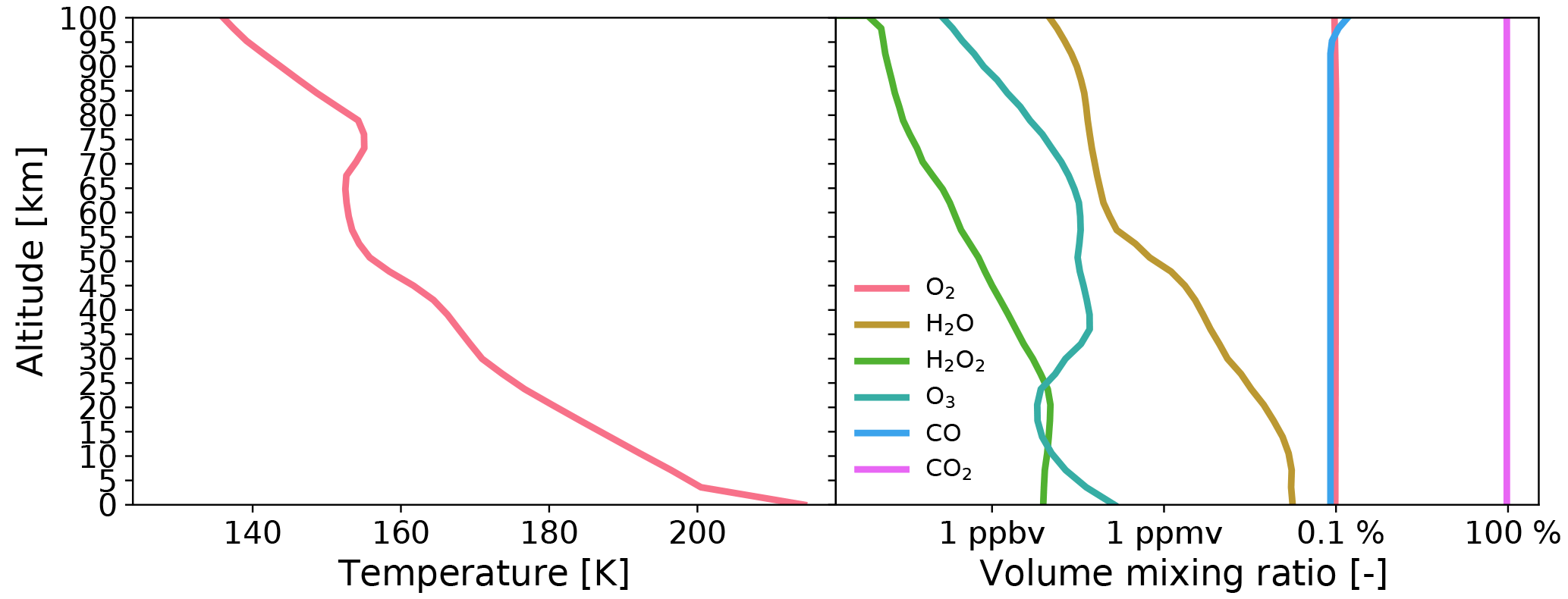
The standard scenario atmosphere is from daytime simulations by Laboratoire de Météorologie Dynamique's global circulation model (Forget et al., 1999) for a solar angle of 0∘. The temperature and volume mixing ratio profiles for key species are shown in Fig. 2. The magnetic field is set to a constant 1 µT throughout the transfer, pointing along the line of sight of the transfer. We expect there to be large variations in some gases (i.e., gaseous water, ozone, and hydrogen peroxide) and in the strength of the magnetic field. In order to demonstrate how the error estimation changes as the forward model scenario changes, we perform the simulations at a 100 times lower volume mixing ratio of these gases and of the magnetic field. In this reduced case, we still keep the temperature and molecular oxygen mixing ratios the same as in the standard scenario. We do not set the wind speed in any scenario but perform retrievals of it from analytical expressions of its Jacobian.
A spectroscopic suite suitable for Mars was developed by Buehler et al. (2018), which we use for our simulations. It computes pressure broadening and shifting per atmospheric species rather than from a predefined atmospheric composition. We also use the carbon dioxide collision-induced absorption from Gruszka and Borysow (1997) as the continua shown in Fig. 3. These continua are key to low-altitude limb measurements and are the main reason we are focusing on the 400 GHz range rather than higher frequencies. Note that the continua are effectively twice as strong as normal since we will not suppress the lower or upper sidebands. A big problem with these continua is that they are only defined down to a temperature of 200 K. For lower temperatures, we simply extrapolate to these using the Gruszka and Borysow (1997) code by ignoring the warnings. Despite these issues, we still choose to include the continua since ignoring a potential 20–120 K signal would be catastrophic for the science of the mission. Clearly, the carbon dioxide continua have to be studied more for Mars atmospheric conditions since their influence is notably strong. Even if our extrapolation is the cause of most of the absorption that we see (because of some model artifact at lower temperatures), it is necessary to confirm that this is the case and to limit the influence of the continua.
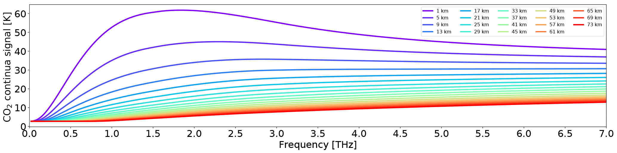
Figure 3Limb pencil view simulation of Mars considering only the carbon dioxide continua. Pencil tangent altitudes are indicated by the legend. The increase in the signal at higher altitudes and higher frequency is probably a consequence of the extrapolation of the model parameters.
2.4 Error analysis
We use the optimal estimation method described by Rodgers (2000) to predict at what level of precision and resolution we will be able to measure atmospheric parameters. This is done by assuming a linear error. Errors tend to be linear near the target even if the retrieval process or underlying physics is non-linear. The computed error is from
where Sa is the a priori covariance matrix, J is the Jacobian matrix, Se is a diagonal radiance error covariance matrix, and ey is a Gaussian realization of the measurement error. This realization is repeated a number of times to estimate the error on retrieved parameters. The measurement error covariance is set to be diagonal, having the square of the standard deviation of the measurement error at each point. For most of the simulations below, we assume a diagonal a priori covariance matrix. For the one figure where we do not assume this at the end, the correlation of this matrix is assumed to decrease exponentially the further the distance is from the diagonal, as described by Eriksson et al. (2005), and the correlations between retrieved parameters (i.e., wind, temperature, magnetic field strength, O2, H2O, H2O2, and O3 volume mixing ratios) are still assumed to be zero. The a priori variance at each altitude level is from a standard deviation of the molecular oxygen mixing ratio of 100 ppmv, of the gaseous water mixing ratio of 1 ppmv, of the hydrogen peroxide and ozone mixing ratios of 10 ppbv, of the magnetic field strength of 10 µT, of the temperature of 10 K, and of the wind speed of 100 m s−1. These numbers were chosen because they are the closest order of magnitude standard deviations that produce a clear measurement response for each model parameter in the limb-scanning simulations at 1 s integration time. For some of these parameters, we will discuss what happens to the error estimations by increasing the standard deviation by 1 order of magnitude. The measurement response is defined as
where u is a vector of ones, and A is the averaging kernel. We define a clear measurement response as max(r)>0.8. The trace of A gives the degrees of freedom of the retrieval system.

Figure 4Simulated signal for the sensor. The signal unit is in Planck-equivalent brightness temperature as expected with the sensor calibrated to have half of its measured signal from each sideband. Panel (a) shows the simulated limb-scanning geometry for several tangent altitudes (used in later figures). The legend contains the tangent altitudes. Panel (b) shows the simulated nadir-staring mode signal (also used in later figures).
Note that the shape of the averaging kernels gives the altitude range where the measurements are sensitive to the atmospheric parameters, a combination of the instrument's statistical and physical vertical resolution. The degrees of freedom of the averaging kernel give a rough estimation of how many distinct parameters can be set over the entire profile altitude range, given the statistical constraints. A reduction in the degrees of freedom by, e.g., assuming a larger statistical correlation distance or by integrating the signal over a wider vertical slice of the atmosphere, should be followed by an increase in the precision of the retrieved parameter at the cost of a loss in vertical resolution. It is also possible to increase the precision of the retrieved model parameters by increasing the integration time to reduce the measurement noise. This has the cost of reducing the spatial resolution either vertically or horizontally. We will not consider this type of reduced resolution in this work, partly because such a reduction can be done by averaging measurements a posteriori so long as the original data are available in a high time resolution. The only test of resolution versus precision we make in this work is one where we vary the a priori correlation distance. Although a very crude estimation, it serves the purpose of finding a limit to the precision.
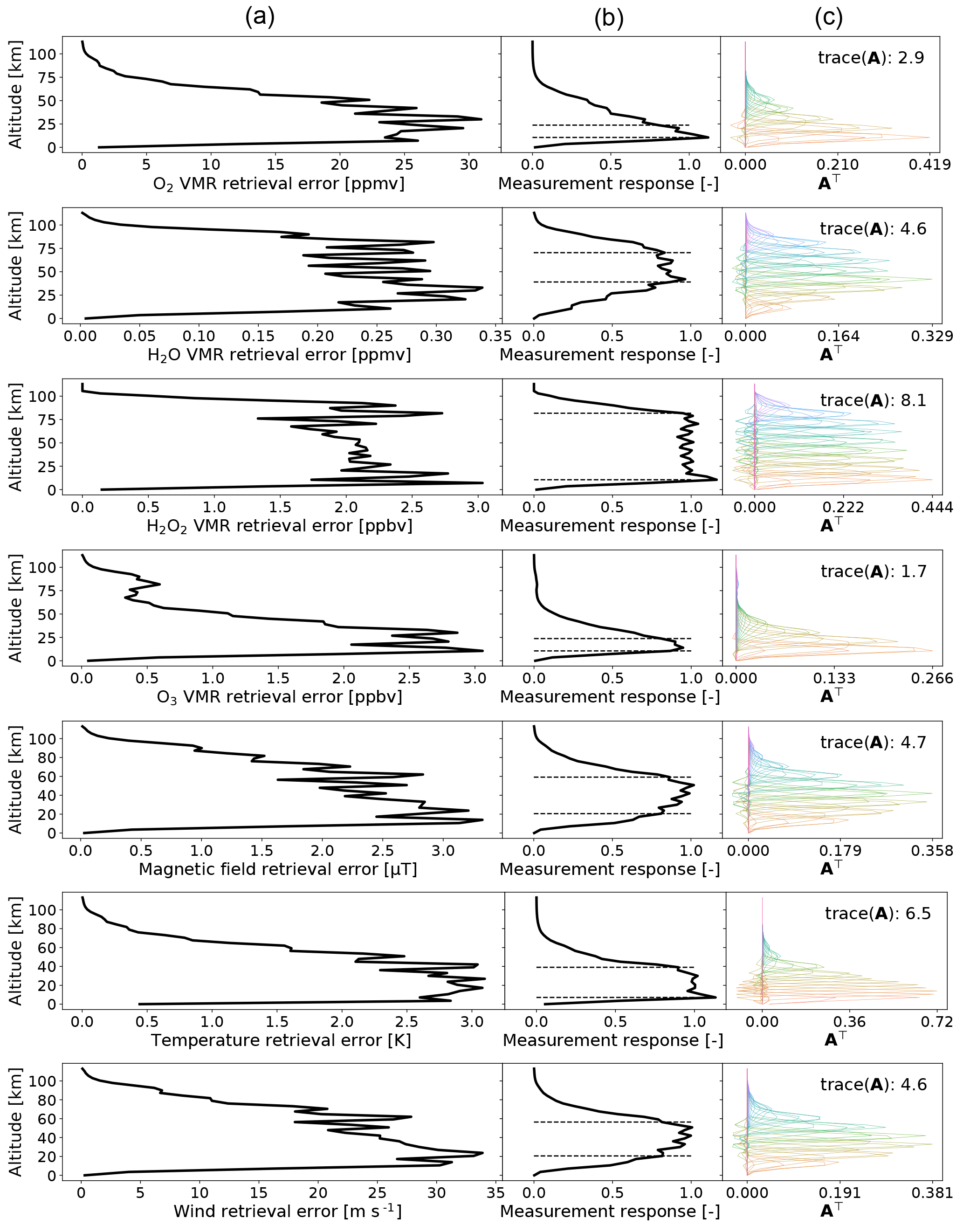
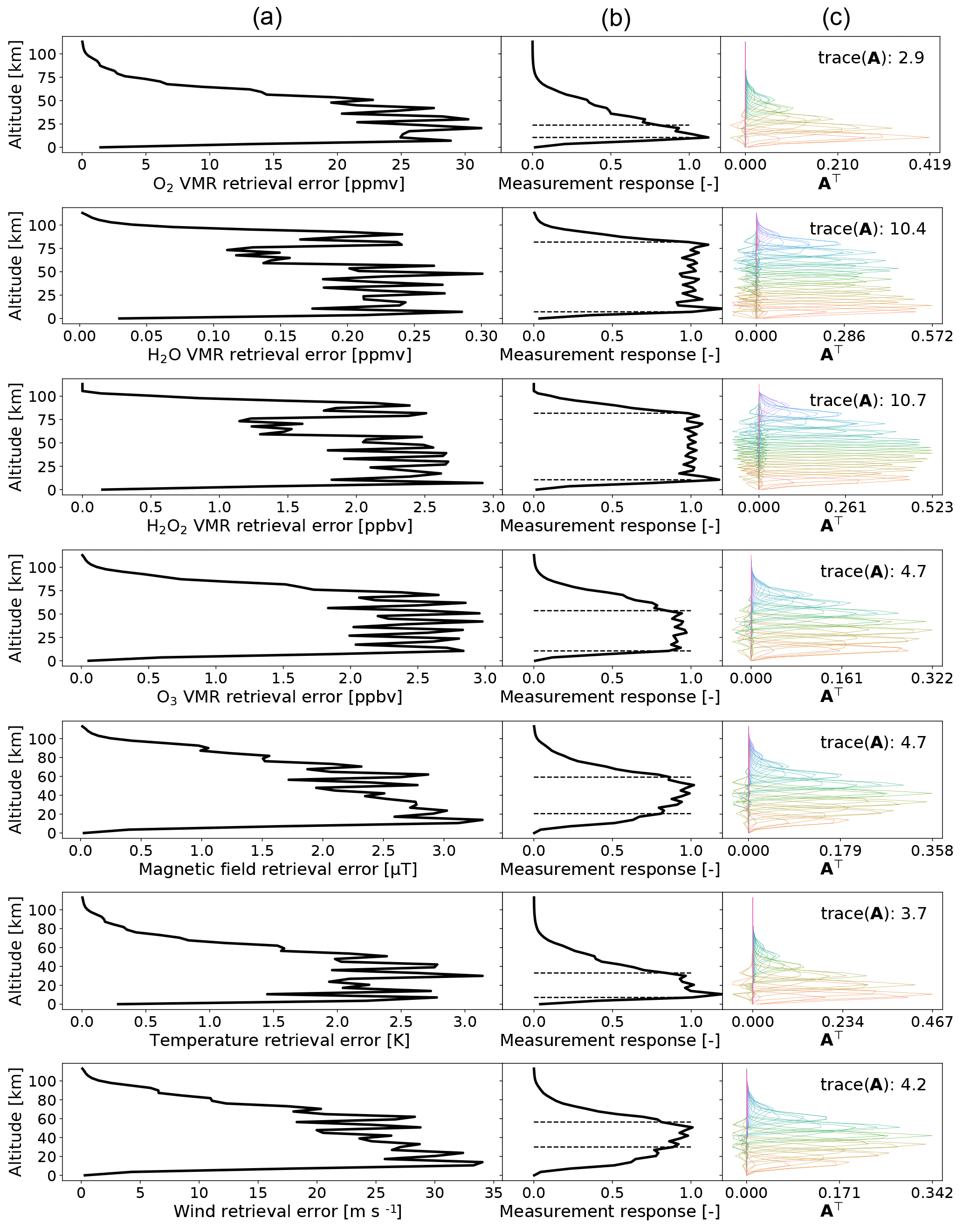
Figure 5Forward model parameter error estimations for the atmosphere of Fig. 2 in limb-scanning mode with 1 s integration time at each of the tangent altitudes of Fig. 4. By columns, column (a) shows the total error estimations and these errors, column (b) shows the measurement response by the solid line with the dashed lines marking the 0.8 level, column (c) shows the transpose of the averaging kernel, color coding its columns and showing its trace or the degrees of freedom of the setup. The rows show the forward model parameters whose retrieval are being simulated, with the top row showing molecular oxygen, the second row showing gaseous water, the third row showing hydrogen peroxide, the fourth row showing ozone, the fifth row showing magnetic field, the sixth row showing temperature, and the last row showing wind speed.
This section gives the forward simulation results and the estimated errors on the retrieved parameters. The first subsection shows the simulated signal in the frequency range we are working in. The next subsection presents the error estimates for limb-scanning observations with a satellite altitude at 400 km for the presented signal and for a signal with 100 times less gaseous water, hydrogen peroxide, and ozone, and with a 100 times weaker magnetic field. The error estimations are from a 1 s long integration time per tangent altitude with all tangent profile used to make up the inputs to Eq. (1) for the error estimations. The next subsection also presents nadir-staring error estimations. We set the integration time to 1 h in nadir-staring mode to reduce the signal-to-noise ratio.
3.1 Modeled sensor signal
The simulated signal from 486.65 to 487.65 GHz and from 475.65 to 474.65 GHz is shown in Fig. 4. The signal shows two hydrogen peroxide absorption lines at 475.20 and 487.20 GHz, a single molecular oxygen absorption line at 487.25 GHz, a single ozone absorption line at 487.35 GHz, and a single gaseous water absorption line near the edge at 474.69 GHz. The limb view signal from molecular oxygen is saturated at the lowest tangent altitude (peaks of 95 K in the double-sideband view), but its signal is more reduced at higher altitudes. The gaseous water signal is also saturated at lower tangent altitudes but weakens greatly at higher tangent altitudes. The ozone signal is weak, about 5 K in strength at low altitudes, due to Ozone's consistently high mixing ratio at higher altitudes. The hydrogen peroxide signal is also weak, but much stronger than the ozone signal, at 10 K at low altitudes, but its strength decreases more rapidly at higher altitudes.
3.2 Error estimations
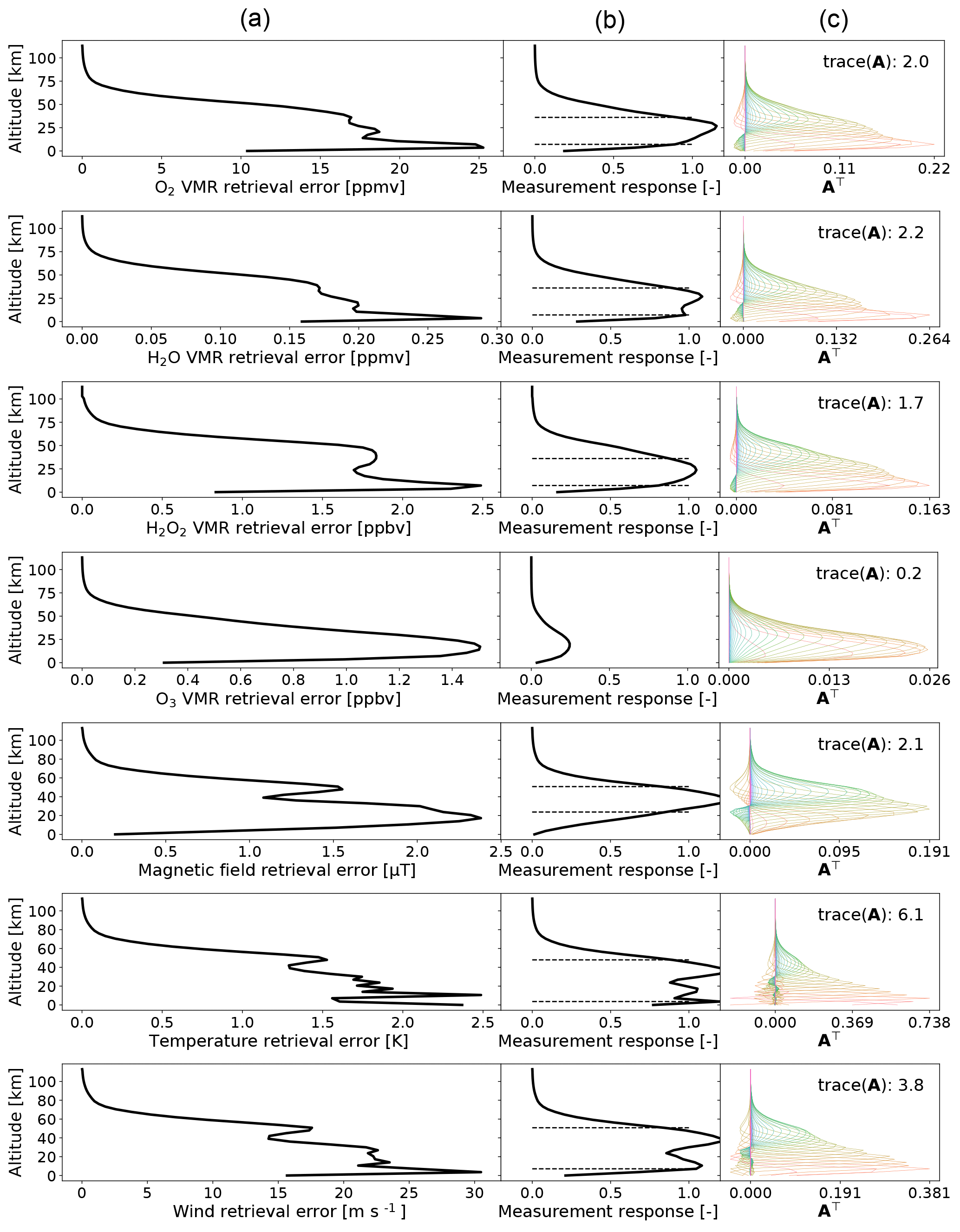
The estimated errors on the forward model parameters for limb-scanning observations are shown in Fig. 5 for a single second of integration time pointing at each of the tangent altitudes of Fig. 4. In addition to the signal in Fig. 4, we also present a case in Fig. 6 where the gaseous water, the hydrogen peroxide, and the ozone volume mixing ratios, as well as the magnetic field strength, are reduced by a factor of 100. Below, for simplicity, the atmosphere with less water is called “dry” and the atmosphere with more water is called “wet”. The estimated errors on the forward model parameters for nadir-staring mode are shown in Fig. 7 for a full 1 h of integration time.
-
In terms of molecular oxygen, expected error levels are of 25 ppmv with good measurement response from 10 to 30 km in the limb-scanning mode. In nadir-staring mode, the altitude range of good measurement response extends from 10 to 40 km, and the expected error is about 15 ppmv. Molecular oxygen is not expected to change at short timescales, so either scenario is good for the purpose of the mission to place a constraint on our knowledge of molecular oxygen variations. Longer integration times in limb-scanning mode, or staring at lower altitudes, could be useful for limiting the vertical profile of the molecule better, especially at lower altitudes. For instance, the very near-surface error achieves good measurement response by merely increasing the integration time to 2 s staring every 10 km from 5 to 35 km.
-
In terms of gaseous water, reducing the gaseous water content increases sensitivity at lower altitudes, as the line absorption is no longer saturated. In limb-scanning mode, the expected error is around 0.2 ppmv, with a range of good measurement response from 40 to 70 km for a wet atmosphere and from 10 to 80 km in a dry atmosphere. In nadir-staring mode, the measurement response is good, from 10 to 40 km, with similar levels of error to those estimated for the limb-scanning mode. To have a good measurement response near the surface for a single profile in a wet atmosphere, the a priori standard deviation of water can be increased by an order of magnitude, which yields an error estimation of about 3 ppmv and good measurement response from the ground to 40 km (not shown).
-
In terms of hydrogen peroxide, in limb-scanning mode, hydrogen peroxide has expected errors around 2 ppbv in both wet and dry atmospheres. Also, the good measurement response altitude range is from 10 to 80 km in both scenarios. The estimated error is similar in the nadir-staring mode, but the altitude range is reduced from 10 to 40 km. An estimated error of 2 ppbv is about 20 % of the total hydrogen peroxide content in the standard wet atmosphere. Since the species abundances are expected to be increased by dust storms, this error should be good enough to characterize its production and destruction inside said storms.
-
In terms of ozone, the instrument is not sensitive to ozone in nadir-staring mode. In limb-scanning mode, the error is expected to be about 2 ppbv. For the wet atmosphere, the good measurement response range is limited to 10 to 30 km. The dry atmosphere offers a much greater responsive measurement range from 10 to 60 km. The wet atmosphere scenario has about 50 ppbv in an altitude range around 50 km, so an error at 2 ppbv is good enough to see variations at high altitudes. Closer to the surface, the ozone mixing ratio increases to above 100 ppbv, but our instrument will only be sensitive for a single profile measurement at those altitudes if the atmosphere is dry and we keep the current constraints. It is possible to improve the sensitivity, e.g., by increasing the standard deviation of ozone in the a priori matrix by 1 order of magnitude. Doing that, the estimate error increases to about 25 ppbv and near-surface altitudes have good measurement response.
-
In terms of magnetic field strength, the error is not affected by the wetness of the atmosphere. For the limb-scanning mode scenario, the estimated error is about 2.5 µT in the altitude range from 20 to 60 km. In nadir-staring mode, the error is expected at 1.5 µT from 20 to 50 km. Note that the magnetic field is not changing over time but is from sources frozen into the crust. So many subsequent orbits can be used to limit the strength of the magnetic field more strongly. The sensor measures circular polarization, so only when the magnetic field is pointing at the sensor will there be a strong signal. For nadir-staring mode, this limits us to the stronger magnetic field areas, which cover a relatively small area. So, to achieve the error here, many subsequent orbits must observe the area. For limb-scanning mode, combining the measurements above a single tangent profile from different azimuth angles will improve the precision even more than shown in our figures. Finally, the molecular oxygen profile in our simulations consists of almost 50 % less molecular oxygen than has previously been measured because these are produced by the circulation model. A 40 % increase in molecular oxygen in our simulations means that the estimated error is reduced by about a third of the error estimates given here.
-
In terms of temperature, in limb-scanning mode, the temperature error estimated for a single profile is about 2 to 2.5 K, with good measurement response from 10 to 40 km. In nadir-staring mode, the temperature error estimation is about 1.5 K, with good measurement response from the ground to 50 km.
-
In terms of wind speed, the wind speed error is estimated from 20 to 25 m s−1 depending on atmospheric wetness, for good measurement response at an altitude range of approximately 20 to 60 km. In nadir-staring mode, wind speed errors are about 20 m s−1, with a good measurement response from 10 to 60 km. The vertical wind speed will not be this strong along the path of observations in nadir-staring mode, so attempting to retrieve the wind parameter with our instrument in nadir observations will not be useful.
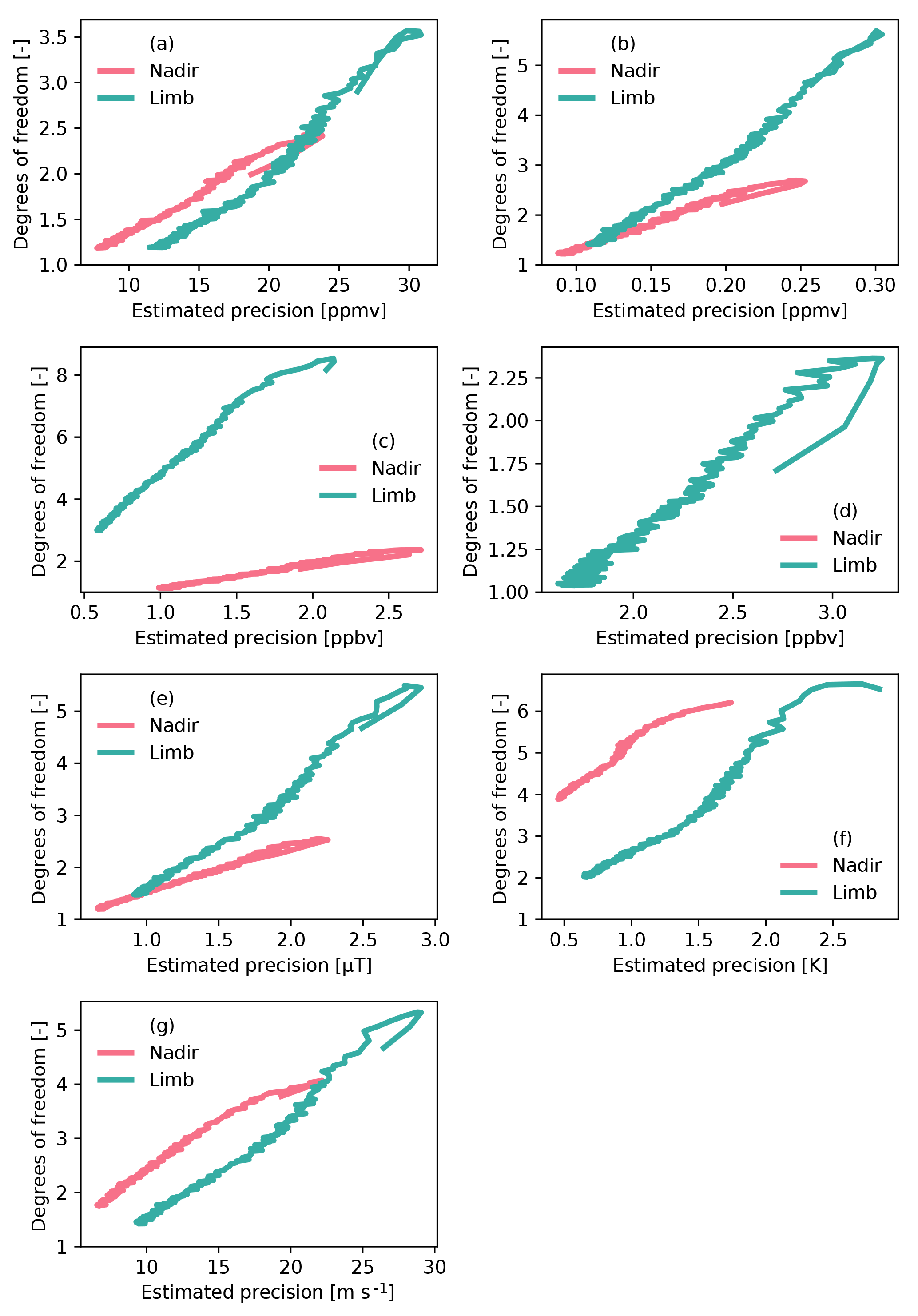
Figure 8Estimated precision versus degrees of freedom (DOFs) by increasing the correlation distance all the way to 1000 km (not shown). Panel (a) is for molecular oxygen. Panel (b) is for gaseous water. Panel (c) is for hydrogen peroxide. Panel (d) is for ozone. Panel (e) is for the magnetic field strength. Panel (f) is for the temperature. Panel (g) is for the wind speed. The legends indicate the observation strategy as used for Figs. 5 or 7. The estimated precisions are the mean over the range of max(r)>0.8, so the ozone panel lacks a line for nadir-staring mode since it is never sensitive at the a priori standard deviations presented in the subsection on error analysis. Note that the solid line goes from shorter correlation distance tending towards higher degrees of freedom to longer correlation distances tending towards lower degrees of freedom. The “hook” that appears on the right-hand side of some of the lines is from correlation distances much shorter than the antenna resolution.
3.3 On vertical resolution versus precision
An estimation of the vertical resolution versus precision can be had by letting the correlation distance increase to large distances. In Fig. 8, we let the correlation distance vary from a diagonal a priori matrix to 1000 km for both nadir-staring and limb-scanning simulations. The figure shows the degrees of freedom of the averaging kernel at these different correlation distances versus the precision in the range where the measurement response is above 80 %. This way, the figure indicates that what we are trading for increased precision is lower degrees of freedom. Lower correlation distances tend to have more degrees of freedom. Since we discuss the uncorrelated case in precious subsection, we limit the discussion below to longer correlation distances, where the degrees of freedom are reduced. These represents a scenario where we assume that the state of the atmosphere at one level is highly correlated with that at every other level. This is a somewhat crude way to reduce the degrees of freedom of the problem, but it serves as an estimate of the error at a lower vertical resolution. For molecular oxygen, this highly correlated state reduces the estimated errors in the nadir-staring mode to about 10 ppmv and in the limb-scanning mode to about 15 ppmv. For gaseous water, the highly correlated state reduces the error estimation to 0.1 ppmv for both nadir-staring and limb-scanning modes. For hydrogen peroxide, the estimated errors are reduced in the highly correlated state to about 1 ppbv in nadir-staring mode and to 0.5 ppbv in limb-scanning mode. The limb-scanning mode retains more than 1 degree of freedom. For ozone, limb-scanning mode errors remain at about 2 ppbv in the highly correlated state, as its degrees of freedom are low to begin with for the uncorrelated a priori covariance matrix. The magnetic field in the highly correlated state has limb-scanning mode estimated errors at 1 µT and in nadir-staring mode at 0.5 µT. Since the magnetic field is highly correlated with vertical distance, these numbers might better represent the precision at which we can retrieve the magnetic field strength from a single profile than the errors estimated in the previous subsection. The temperature error estimation in the highly correlated case retains degrees of freedom in both nadir-staring and limb-scanning modes, meaning the retrieval system does not allow the trade that we are after. The errors are expected to be about 0.5 K. The wind speed errors are expected to be around 5 to 10 m s−1 in the highly correlated case.
We present a feasibility study for a submillimeter instrument on a small Mars mission currently under construction. The instrument will be able to measure several atmospheric species crucial for understanding Martian molecular oxygen, gaseous water, hydrogen peroxide, and ozone at low errors. In addition to these, the instrument will be able to limit the crustal magnetic field and get the meteorological parameters of temperature and wind speed. The expected measurement errors before spatial and temporal averaging are 15 to 25 ppmv for the molecular oxygen mixing ratio, 0.2 ppmv for the gaseous water mixing ratio, 2 ppbv for the hydrogen peroxide mixing ratio, 2 ppbv for the ozone mixing ratio, 1.5 to 2.5 µT for the magnetic field strength, 1.5 to 2.5 K for the temperature profile, and 20 to 25 m s−1 for the horizontal wind speed. These error ranges are well within the range needed to push the boundary of Mars knowledge.
The data, the model, and related tools used in this study can be examined by subversion and/or git via http://www.radiativetransfer.org (last access: 13 December 2018). The data are in the subversion repository https://arts.mi.uni-hamburg.de/svn/rt/arts-xml-data/trunk/ (last access: 13 December 2018) and the model is in the subversion repository https://arts.mi.uni-hamburg.de/svn/rt/arts/trunk (last access: 13 December 2018).
RL prepared the manuscript with input from all co-authors. He also performed the underlying forward simulations and retrievals. YK initiated the concept as the leader of the project. TK provided to discussions about the Martian atmosphere. SS manages the general sensor design process. TY helped with discussions on the forward simulations and provided insights on electro-chemistry of hydrogen peroxide. HM helped with the general backend designs. YH provided the polarization feedhorn design. TN contributed with the antenna design. SN provides towards the platform design. PH provided expertise on the chirp transform spectrometer.
The authors declare that they have no conflict of interest.
Richard Larsson was funded by DFG project HA3261/9-1 in the later parts of the study, after the
initial review.
Edited by: Maria Genzer
Reviewed by: two anonymous referees
Atreya, S., Wong, A.-S., Renna, N., Farrell, W., Delory, G., Sentman, D., Cummer, S., Marshall, J., Rafkin, S., and Catling, D.: Oxidant Enhancement in Martian Dust Devils and Storms: Implication for Life and Habitability, Astrobiology, 6, 439–450, 2006. a
Buehler, S. A., Mendrok, J., Eriksson, P., Perrin, A., Larsson, R., and Lemke, O.: ARTS, the Atmospheric Radiative Transfer Simulator – version 2.2, the planetary toolbox edition, Geosci. Model Dev., 11, 1537–1556, https://doi.org/10.5194/gmd-11-1537-2018, 2018. a, b
Carleton, N. P. and Traub, W. A.: Detection of molecular oxygen on Mars, Science, 177, 988–992, 1972. a
Delory, G., Farrell, W., Atreya, S., Renna, N., Wong, A.-S., Cummer, S., Sentman, D., Marshall, J., Rafkin, S., and Catling, D.: Oxidant Enhancement in Martian Dust Devils and Storms: Storm Electric Fields and Electron Dissociative Attachment, Astrobiology, 6, 450–462, 2006. a
Eriksson, P., Jiménez, C., and Buehler, S. A.: Qpack, a general tool for instrument simulation and retrieval work, J. Quant. Spectrosc. Ra., 91, 47–64, https://doi.org/10.1016/j.jqsrt.2004.05.050, 2005. a
Eriksson, P., Buehler, S. A., Davis, C. P., Emde, C., and Lemke, O.: ARTS, the atmospheric radiative transfer simulator, Version 2, J. Quant. Spectrosc. Ra., 112, 1551–1558, 2011. a
Forget, F., Hourdin, F., Foumier, R., Hourdin, C., and Talagran, O.: Improved general circulation models of the Martian atmosphere from the surface to above 80 km, J. Geophys. Res., 104, 155–175, 1999. a
Gruszka, M. and Borysow, A.: Roto-Translational Collision-Induced Absorption of CO2 for the Atmosphere of Venus at Frequencies from 0 to 250 cm−1, at Temperatures from 200 to 800 K, Icarus, 129, 172–177, https://doi.org/10.1006/icar.1997.5773, 1997. a, b
Hartogh, P.: High-resolution chirp transform spectrometer for middle atmospheric microwave sounding, https://doi.org/10.1117/12.301141, 1997. a
Hartogh, P. and Hartmann, G. K.: A high-resolution chirp transform spectrometer for microwave measurements, Meas. Sci. Technol., 1, 592 pp., available at: http://stacks.iop.org/0957-0233/1/i=7/a=008 (last access: 10 December 2018), 1990. a
Hartogh, P. and Osterschek, K.: Multiband chirp transform spectrometer for the microwave remote sensing of middle atmospheric trace gases, Proc. SPIE, 2583, 2583–2583–8, https://doi.org/10.1117/12.228573, 1995. a
Hartogh, P., Jarchow, C., Lellouch, E., Val-Borro, M., Rengel, M., Moreno, R., Medvedev, A., Sagawa, H., Swinyard, B., Cavalié, T., Lis, D., Błȩcka, M., Banaszkiewicz, M., Bockelée-Morvan, D., Crovisier, J., Encrenaz, T., Küppers, M., Lara, L., Szutowicz, S., Vandenbussche, B., Bensch, F., Bergin, E. A., Billebaud, F., Biver, N., Blake, G., Blommaert, J., Cernicharo, J., Decin, L., Encrenaz, P., Feuchtgruber, H., Fulton, T., de Graauw, T., Jehin, E., Kidger, M., Lorente, R., Naylor, D., Portyankina, G., Sánchez-Portal, M., Schieder, R., Sidher, S., Thomas, N., Verdugo, E., Waelkens, C., Whyborn, N., Teyssier, D., Helmich, F., Roelfsema, P., Stutzki, J., LeDuc, H., and Stern, J.: Herschel/HIFI observations of Mars: first detection of O2 at submillimetre wavelengths and upper limits on HCl and H2O2, Astron. Astrophys., 521, L49, https://doi.org/10.1051/0004-6361/201015160, 2010. a
Kasai, Y., Sagawa, H., Kuroda, T., Manabe, T., Ochiai, S., Kikuchi, K., Nishibori, T., Baron, P., Mendrok, J., Hartogh, P., Murtagh, D., Urban, J., von Schéele, F., and Frisk, U.: Overview of the Martian atmospheric submillimetre sounder FIRE, Planet. Space Sci., 63-64, 62–82, 2012. a, b
Larsson, R., Ramstad, R., Mendrok, J., Buehler, S. A., and Kasai, Y.: A Method for Remote Sensing of Weak Planetary Magnetic Fields: Simulated Application to Mars, Geophys. Res. Lett., 40, 5014–5018, 2013. a
Larsson, R., Buehler, S. A., Eriksson, P., and Mendrok, J.: A treatment of the Zeeman effect using Stokes formalism and its implementation in the Atmospheric Radiative Transfer Simulator (ARTS), J. Quant. Spectrosc. Ra., 133, 445–453, 2014. a
Larsson, R., Milz, M., Eriksson, P., Mendrok, J., Kasai, Y., Buehler, S. A., Diéval, C., Brain, D., and Hartogh, P.: Martian magnetism with orbiting sub-millimeter sensor: simulated retrieval system, Geosci. Instrum. Method. Data Syst., 6, 27–37, https://doi.org/10.5194/gi-6-27-2017, 2017. a
Larsson, R., Lankhaar, B., and Eriksson, P.: Updated Zeeman effect splitting coefficients for molecular oxygen in planetary applications, J. Quant. Spectrosc. Ra., 224, 431–438, https://doi.org/10.1016/j.jqsrt.2018.12.004, 2018. a
Mahaffy, P. R., Webster, C. R., Atreya, S. K., Franz, H., Wong, M., Conrad, P. G., Harpold, D., Jones, J. J., Leshin, L. A., Manning, H., Owen, T., Pepin, R. O., Squyres, S., Trainer, and Team, M. S.: Abundance and Isotopic Composition of Gases in the Martian Atmosphere from the Curiosity Rover, Science, 341, 263–266, 2013. a
Paganini, L. and Hartogh, P.: Analysis of nonlinear effects in microwave spectrometers, J. Geophys. Res.-Atmos., 114, D13305, https://doi.org/10.1029/2008JD011141, 2009. a
Rodgers, C. D.: Inverse methods for atmospheric sounding: Theory and practice, vol. 2, World Scientific Publishing Co. Pte. Ltd., 2000. a
Sandel, B., Gröller, H., Yelle, R., Koskinen, T., Lewis, N., Bertaux, J.-L., Montmessin, F., and Quémerais, E.: Altitude profiles of O2 on Mars from SPICAM stellar occultations, Icarus, 252, 154–160, https://doi.org/10.1016/j.icarus.2015.01.004, 2015. a, b, c
Urban, J., Dassas, K., Forget, F., and Ricaud, P.: Retrieval of vertical constituents and temperature profiles from passive submillimeter wave limb observations of the Martian atmosphere: a feasibility study, Appl. Optics, 44, 2438–2455, https://doi.org/10.1364/AO.44.002438, 2005. a
Villanueva, G. and Hartogh, P.: The High Resolution Chirp Transform Spectrometer for the Sofia-Great Instrument, Exp. Astron., 18, 77–91, https://doi.org/10.1007/s10686-005-9004-3, 2004. a
Villanueva, G. L., Hartogh, P., and Reindl, L. M.: A digital dispersive matching network for SAW devices in chirp transform spectrometers, IEEE T. Microw. Theory, 54, 1415–1424, https://doi.org/10.1109/TMTT.2006.871244, 2006. a
Zeeman, P.: On the Influence of Magnetism on the Nature of the Light Emitted by a Substance, Astrophys. J., 5, 332–347, https://doi.org/10.1086/140355, 1897. a