The combined processing of geomagnetic intensity vector projections and absolute magnitude measurements

Getmanov, Victor G.; Gvishiani, Alexei D.; Sidorov, Roman V.

doi:https://doi.org/10.5194/gi-8-209-2019

Articles | Volume 8, issue 2

https://doi.org/10.5194/gi-8-209-2019

Articles | Volume 8, issue 2

Research article

22 Aug 2019

Research article |

| 22 Aug 2019

The combined processing of geomagnetic intensity vector projections and absolute magnitude measurements

Victor G. Getmanov, Alexei D. Gvishiani, and Roman V. Sidorov

Abstract

A method for the combined processing measurements of the projections and the absolute magnitudes of geomagnetic field intensity vectors, based on mathematical technology of local approximation models, is proposed. The approach realized in this paper, based on the proposed method, provides an increase in quality of the measurements of the projections of the geomagnetic intensity vector. An algorithm for the two-stage combined processing of the measurements of projections and absolute magnitudes of geomagnetic field intensity vectors is developed. The operation of the combined processing algorithm was tested on models and observatory measurements. The estimates of the combined processing algorithm errors were obtained using statistical modelling. The reduction of the root-mean-square error values was achieved for the estimates of the projections of geomagnetic field intensity vectors.

Please read the corrigendum first before continuing.

Download & links

Article (PDF, 764 KB)

Notice on corrigendum
The requested paper has a corresponding corrigendum published. Please read the corrigendum first before downloading the article.
Article (764 KB)

Corrigendum

Download & links

The requested paper has a corresponding corrigendum published. Please read the corrigendum first before downloading the article.

How to cite

How to cite.

Dates

Received: 20 Jun 2018 – Discussion started: 06 Nov 2018 – Revised: 25 Jul 2019 – Accepted: 27 Jul 2019 – Published: 22 Aug 2019

1 Introduction

In this article, a method and an algorithm for combined processing measurements of the components (projections and the absolute magnitudes) of geomagnetic field intensity vectors is proposed. The approach realized in the paper, based on the proposed method, provides an increase in quality of the measurements of the projections of the geomagnetic intensity vector. The considered measurements are carried out by INTERMAGNET observatories equipped with systems of vector and scalar magnetometers; the definitive type data are used, containing systematic errors equal to zero (Mandea and Korte, 2011; INTERMAGNET, 2018). The measurement errors of vector and scalar magnetometers are represented by random, normally distributed errors with zero expectation and a predetermined variance. As usual, the measurement errors of the projections of geomagnetic field intensity vectors are significantly larger than the ones of the absolute vector magnitudes performed by the mentioned measurement devices. The formulation of the problem of reducing the noise root-mean-square (RMS) error values in the geomagnetic field intensity projection measurements is due to combined processing of the values of all its components.

In the following research, the following steps are outlined:

A method for combined processing of the measurements of projections and absolute magnitudes of geomagnetic field intensity vectors is formulated, based on formation of the sequences of piecewise-constant local models followed by their weighted averaging;
A two-stage algorithm for combined processing of the measurements of projections and absolute magnitudes of geomagnetic field intensity vectors is developed;
Testing of the algorithm on model and observatory data is performed;
The estimates of the algorithm errors, calculated using statistical modelling, are presented; the reduction of the RMS noise errors for the estimates of the geomagnetic field vector projections is proved.

The material in this research paper is intended for specialists (magnetologists) engaged in digital processing of geomagnetic field measurements. The need to reduce noise errors in estimates of the projections of the geomagnetic field intensity vectors measured by vector magnetometers arises in a number of technical and scientific applications. For instance, technogenic disturbances can affect the geomagnetic observatory hardware, affecting vector and scalar magnetometers differently: as a rule, the noise errors from vector magnetometers occurring due to such interference are greater than the noise errors from scalar magnetometers. The decrease in noise errors from vector magnetometers is necessary, e.g. for calculation of the gradients of the projections of the geomagnetic field intensity vectors in the navigation problems.

Nowadays the reduction of errors for vector magnetometers (with certain assumptions) is achieved using optimization of the calibration from scalar magnetometers (Merrayo et al., 2000; Olsen et al., 2003) or refinement of calibration characteristics (Soborov et al., 2008) based on special mathematical processing. In the measurement systems considered in this paper, in fact, parallel measurements are performed; a possible algorithm providing the decrease in errors for such measurements can be formed based on Kalman filters (Shakhtarin, 2008). However, due to the peculiarities of this problem, the construction of the resulting non-linear filters is associated with certain problems due to the inaccuracies of linearization and the accepted hypothesis concerning the type of initial intensity vector function. In other research (Soloviev et al., 2018), joint processing of vector and scalar magnetometer measurements aimed at improving the calibration accuracy of the so-called baseline, which only indirectly provides the considered reduction in errors. The combined processing of measurements of projections and absolute magnitudes of geomagnetic field intensity vectors proposed in this paper is significantly free from the mentioned problems.

2 A method for combined processing of measurements of projections and absolute magnitudes of geomagnetic field intensity vectors

Let H₁(Ti), H₂(Ti), H₃(Ti), and $H_{0} (T i) = \sqrt{H_{1}^{2} (T i) + H_{2}^{2} (T i) + H_{3}^{2} (T i)}$ be the initial functions for the projections and absolute magnitudes of the geomagnetic field intensity vectors; we assume that Y₁(Ti), Y₂(Ti), Y₃(Ti), and Y₀(Ti) are their values registered by vector and scalar magnetometers, $i = 0, 1, \dots, N_{f} - 1$ ; the sampling interval T=1 s; 1 s measurements from INTERMAGNET observatories are analysed in this study. For $n = 0, \dots, 3$ , we represent the noise errors of the measurement values W_n(Ti) in the form of uncorrelated, normally distributed random values with zero mathematical expectations and some variances. Such a representation of errors is, to a large extent, valid for cases of large technogenic noises that can occur when geomagnetic measurements are carried out. We consider, with some assumptions, that the spectrum of random components for the functions of the geomagnetic field is concentrated almost entirely in the low-frequency domain, and the spectrum of random measurement errors is concentrated in the high-frequency domain.

We assume that the measurements, the initial functions, and the errors are related by linear additive dependences:

Y_{n} (T i) = H_{n} (T i) + W_{n} (T i), n = 0, \dots, 3 .

Using the specified observation values Y_n(Ti), we demand the determination of the estimates $Y_{1}^{\circ} (T i)$ , $Y_{2}^{\circ} (T i)$ , and $Y_{3}^{\circ} (T i)$ , where $i = 0, 1, \dots, N_{f} - 1$ , that would be close to the initial functions of the intensity vector projections. We perform the combined processing for the projections and magnitudes of the geomagnetic field intensity vectors in two stages.

At the first stage, on the main interval with the points $i = 0, 1, \dots, N_{f} - 1$ , we introduce the N-point sliding local intervals with limiting points $N_{1_{j}}$ , $N_{2_{j}}$ , and the sliding step N_d as well as the quantity of sliding intervals m₀.

\begin{matrix} (1) & \begin{aligned} N_{1_{j}} = N_{d} (j - 1), N_{2_{j}} = N_{1_{j}} + N - 1, \\ j = 1, \dots, m_{0} . \end{aligned} \end{matrix}

To simplify the considerations, we require the relations of multiplicity mN=N_f and N_dm_d=N; here, if m and m_d are integers, then $m_{0} = m_{d} (m - 1) + 1$ .

For a sliding interval with a number j, we define the model functions of a form $Y_{M_{1}} (c_{1_{j}}, T i)$ , $Y_{M_{2}} (c_{2_{j}}, T i)$ , and $Y_{M_{3}} (c_{3_{j}}, T i)$ ; here, $c_{n_{j}}$ is the vectors of model parameters, n=1, 2, 3. These model functions can be, in particular, polynomial, piecewise constant, piecewise linear, etc. The size of local intervals determines the approximation errors. At small N there will be large fluctuation errors, and at large N there will be large systematic approximation errors.

Based on the above-defined measured values, models, and the maximum likelihood method (Kramer, 1975), we define the local functional S(c_jY_j) which determines the measure of closeness for local measurements and models, similar to Getmanov (2013) as the sum of the four functionals:

\begin{matrix} (2) & \begin{aligned} S_{0} (c_{1_{j}}, c_{2_{j}}, c_{3_{j}}, Y_{0_{j}}) = \\ \sum_{i = N_{1_{j}}}^{N_{2_{j}}} {(Y_{0_{j}} (T i) - \sqrt{\sum_{r = 1}^{3} Y_{M_{r}}^{2} (c_{r_{j}}, T i)})}^{2} \\ S_{n} (c_{n_{j}}, Y_{n_{j}}) = \sum_{i = N_{1_{j}}}^{N_{2_{j}}} {(Y_{n_{j}} (T i) - Y_{M_{n}} (c_{n_{j}}, T i))}^{2}, \\ n = 1, 2, 3, \\ S (c_{j}, Y_{j}) = S_{0} (c_{1_{j}}, c_{2_{j}}, c_{3_{j}}, Y_{0_{j}}) + \sum_{n = 1}^{3} S_{n} (c_{n_{j}}, Y_{n_{j}}) . \end{aligned} \end{matrix}

Here, $c_{j}^{T} = (c_{1_{j}}^{T} c_{2_{j}}^{T}, c_{3_{j}}^{T})$ and $Y_{j}^{T} = (Y_{1_{j}}^{T} Y_{2_{j}}^{T}, Y_{3_{j}}^{T})$ are the parameter and value vectors related to the jth local interval. Taking into account the assumption of errors in measurements, we carry out the identification of the optimal estimates of the model parameters $c_{j}^{\circ}$ using the solutions of the sequence of optimization problems for local functionals:

\begin{matrix} (3) & \begin{aligned} c_{j}^{\circ} = \arg \{S (c_{j}, Y_{j})\}, j = 1, \dots, m_{0}, \\ c^{\circ T} = (c_{1}^{\circ T}, c_{2}^{\circ T}, c_{3}^{\circ T}) . \end{aligned} \end{matrix}

We perform the construction of sliding local models in an obvious way by assuming n=1, 2, 3, and $j = 1, \dots, m_{0}$ .

\begin{matrix} (4) & \begin{aligned} Y_{n_{j}}^{\circ} (T i) = Y_{M_{n}} (c_{n_{j}}^{\circ}, T i), N_{1_{j}} \leq i \leq N_{2_{j}}, \\ Y_{n_{j}}^{\circ} (T i) = 0, 0 \leq i < N_{1_{j}}, N_{2_{j}} < i \leq N_{f} - 1 . \end{aligned} \end{matrix}

At the second stage we introduce the unit functions E_j(Ti), equal to zero outside of local sliding intervals, add them together to get E(Ti), and calculate the sequence of weighting coefficients R(Ti):

\begin{matrix} (5) & \begin{aligned} E_{j} (T i) = 1, N_{1_{j}} \leq i \leq N_{2_{j}}, E_{j} (T i) = 0, \\ 0 \leq i < N_{1_{j}}, N_{2_{j}} < i \leq N_{f} - 1; \\ E (T i) = \sum_{j = 1}^{m_{0}} E_{j} (T i), R (T i) = 1 / E (T i), \\ i = 0, 1, \dots, N_{f} - 1 . \end{aligned} \end{matrix}

Let us perform the weighting averaging using Eq. (5) for the sum of the sliding local model sequence (Getmanov et al., 2015).

\begin{matrix} (6) & Y_{n}^{\circ} (T i) = R (T i) \sum_{j = 1}^{m_{0}} Y_{n_{j}}^{\circ} (T i) \end{matrix}

We calculate the estimates $Y_{n}^{\circ} (T i)$ and $i = 0, 1, \dots, N_{f} - 1$ , where n=1, 2, 3, based on linear operations in Eq. (6) corresponding to the second stage.

The method of combined two-step processing of the values of the projections and the absolute magnitudes of geomagnetic field intensity vectors consists of the sequential execution of the first and second stages in accordance with Eqs. (2)–(6).

3 An algorithm for two-stage processing of measurements of projections and absolute magnitudes of geomagnetic field intensity vectors for piecewise-constant models

Let us build the local intervals using Eq. (1) and define the local models on them as piecewise-constant functions $Y_{M_{n}} (c_{n_{j}}, T i) = c_{n_{j}}$ , $j = 1, \dots, m_{0}$ , and $N_{1_{j}} \leq i \leq N_{2_{j}}$ . In this case it is obvious that the initial functions for geomagnetic field vector projections must be approximately constant at local intervals with duration NT. The local interval can be expanded if we treat piecewise-constant functions as local models. Let us formulate the equation for local functionals:

\begin{matrix} (7) & \begin{aligned} S (c_{j}, Y_{j}) = & \sum_{n = 1}^{3} (\sum_{i = N_{1_{j}}}^{N_{2_{j}}} {(Y_{n_{j}} (T i) - c_{n_{j}})}^{2} \\ + \sum_{i = N_{1_{j}}}^{N_{2_{j}}} {(Y_{0_{j}} (T i) - \sqrt{c_{1_{j}}^{2} + c_{2_{j}}^{2} + c_{3_{j}}^{2}})}^{2}) . \end{aligned} \end{matrix}

We differentiate Eq. (7) with respect to $c_{n_{j}}$ , equate the derivatives to zero, and get the necessary conditions for an extremum in the form of a system of three non-linear algebraic equations as a result:

\begin{aligned} \frac{\partial S (c_{j}, Y_{j})}{\partial c_{n_{j}}} = & \sum_{i = N_{1_{j}}}^{N_{2_{j}}} Y_{n_{j}} (T i) - 2 N c_{n_{j}} \\ + \frac{c_{n_{j}} \sum_{i = N_{1_{j}}}^{N_{2_{j}}} Y_{0_{j}} (T i)}{\sqrt{c_{1_{j}}^{2} + c_{2_{j}}^{2} + c_{3_{j}}^{2}}} = 0, \\ n = 1, 2, 3 . \end{aligned}

In this case, an exact analytical solution to this system is possible. Omitting the calculations, we obtain expressions for local estimates, $j = 1, \dots, m_{0}$ :

\begin{matrix} (8) & \begin{aligned} c_{n_{j}}^{\circ} = \frac{1}{2 N} \\ (1 + \frac{\sum_{r = N_{1_{j}}}^{N_{2_{j}}} Y_{0_{j}} (T r)}{\sqrt{{(\sum_{r = N_{1_{j}}}^{N_{2_{j}}} Y_{1_{j}} (T r))}^{2} + {(\sum_{r = N_{1_{j}}}^{N_{2_{j}}} Y_{2_{j}} (T r))}^{2} + {(\sum_{r = N_{1_{j}}}^{N_{2_{j}}} Y_{3_{j}} (T r))}^{2}}}) \\ \sum_{i = N_{1_{j}}}^{N_{2_{j}}} Y_{n_{j}} (T i), \end{aligned} \end{matrix}

where n=1, 2, 3, and get the piecewise-constant functions for local estimates $Y_{n}^{\circ} (T i) = c_{n_{j}}^{\circ}$ , $N_{1_{j}} \leq i \leq N_{2_{j}}$ , $Y_{n}^{\circ} (T i) = 0$ , $0 \leq i < N_{1_{j}}$ , $N_{2_{j}} < i \leq N_{f} - 1$ , and n=1, 2, 3, using Eq. (8) according to Eq. (4); let us present them as the realization of the first stage.

Weighted averaging of sequences of piecewise-constant local estimates and the calculations of the estimate functions $Y_{n}^{\circ} (T i)$ for the second stage are performed using Eqs. (5) and (6).

4 Testing of the algorithm for combined processing on model and observatory measurements

4.1 Testing on model data

The developed algorithm for combined processing was tested on model measurements. Initial model functions for the projections of the geomagnetic intensity vector $H_{M G_{n}} (T i)$ were presented as quadratic functions; the model function for the absolute vector magnitude $H_{M G_{0}} (T i)$ was calculated based on $H_{M G_{n}} (T i)$ , n=1, 2, 3.

\begin{aligned} H_{M G_{n}} (T i) = a_{0, n} + a_{1, n} T i + a_{2, n} {(T i)}^{2}, \\ H_{M G_{0}} (T i) = \sqrt{H_{M G_{1}}^{2} (T i) + H_{M G_{2}}^{2} (T i) + H_{M G_{3}}^{2} (T i)}, \end{aligned}

and $i = 0, 1, \dots, N_{f} - 1$ . The noise error functions W_n(Ti) and n=0, 1, 2, 3 were modelled using normally distributed values with zero mathematical expectation and the variances $σ_{1}^{2} = σ_{2}^{2} = σ_{3}^{2} = σ^{2}$ and $σ_{0}^{2}$ . The model values of the projections the absolute magnitude of the intensity vector were represented as sums:

\begin{matrix} (9) & \begin{aligned} H_{M_{n}} (T i) = H_{M G_{n}} (T i) + W_{n} (T i), \\ i = 0, 1, \dots, N_{f} - 1, \end{aligned} \end{matrix}

where n=0, 1, 2, 3. The following parameter values for the model functions were assigned: $a_{0, 1} = 30 000$ , $a_{1, 1} = 0.4206$ , $a_{2, 1} = - 0.0040$ , $a_{0, 2} = 4300.4$ , $a_{1, 2} = a_{1, 2} = - 0.4252$ , $α_{2, 2} = 0.0043$ , $a_{0, 3} = 4089.5$ , $a_{1, 3} = 0.5013$ , $α_{2, 3} = - 0.0056$ , and T=1 s. Model measurement values $H_{M_{n}} (T i)$ were the input of Eq. (8) of the algorithm for combined processing based on piecewise-constant models.

The case of local intervals without sliding was considered, with the number of points N, $N_{1 j} = N (j - 1)$ and $N_{2 j} = N_{1 j} + N - 1$ , where $j = 1, \dots, m$ and mN=N_f. The local estimates $H_{n_{j}}^{\circ} = c_{j}^{\circ}$ , where $j = 1, \dots, m$ , were calculated, and the sequences of piecewise constant estimates $H_{L_{n}}^{\circ} (T i)$ , n=1, 2, 3, corresponding to the first processing stage, were formed.

For a sliding local intervals case with the number of points N, the sliding step N_d was selected, as well as the number of sliding local intervals m₀. Local estimates $H_{n_{j}}^{\circ} = c_{j}^{\circ}$ , $j = 1, \dots, m_{0}$ , and the estimates of functions $H_{n_{j}}^{\circ} (T i)$ , where n=1, 2, 3 and $i = 0, 1, \dots, N_{f} - 1$ , corresponding to the first processing stage, were calculated. Next, the second stage was performed where the estimates $H_{S_{n}}^{\circ} (T i)$ were found.

https://www.geosci-instrum-method-data-syst.net/8/209/2019/gi-8-209-2019-f01

Figure 1Results of testing the processing algorithm on model measurement data: 1 – initial model functions, 2 – noised model functions, 3 – first-stage result (piecewise-constant model estimates without sliding), and 4 – second-stage result (estimates with weighted averaging).

Download

For testing, the following values were selected: N_f=96, N=12, m=8, N_d=1, m₀=84, σ=1.0 nT, and σ₀=0.5 nT. In Fig. 1, the calculation results are displayed for $H_{M G_{1}}$ (Fig. 2a) and $H_{M G_{2}}$ (Fig. 2b), $H_{M G_{3}}$ (Fig. 2c); dashed lines with index 1 depict the initial functions for the projections of the geomagnetic field intensity vector $H_{M G_{n}} (T i)$ ; lines with index 2 represent the noised measurements of the projections of the geomagnetic field intensity $H_{M_{n}} (T i)$ ; piecewise-constant lines with index 3 represent the results of the first stage $H_{L_{n}}^{\circ} (T i)$ ; solid lines with index 4 show the estimates $H_{S_{n}}^{\circ} (T i)$ – the second-stage results with weighted averaging.

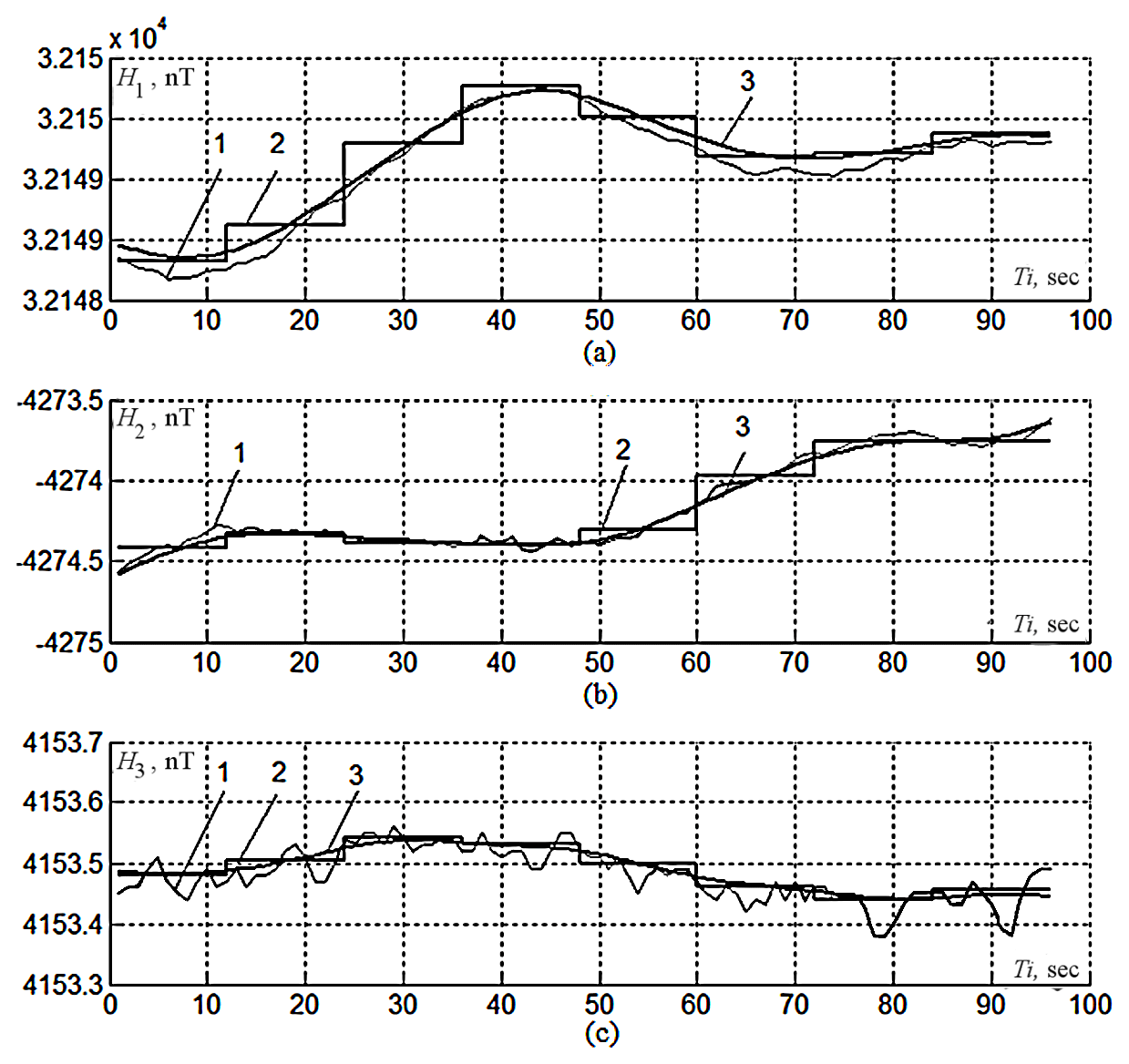
https://www.geosci-instrum-method-data-syst.net/8/209/2019/gi-8-209-2019-f02

Figure 2Results of testing the processing algorithm on observatory measurement data: 1 – initial data, 2 – first-stage result ( piecewise constant model estimates without sliding), and 3 – second-stage result (estimates with weighted averaging with sliding).

Download

The performed testing of the processing algorithm on model data for a number of parameters led to the conclusion that the second stage of processing reduces the RMS of the errors of the first stage by 60 %–80 % on average.

4.2 Testing on real observatory geomagnetic data

The developed algorithm was tested using combined processing of 1 s sampled geomagnetic measurements from the INTERMAGNET observatory MBO (Mbour, Senegal). The measurements were recorded on 2 January 2014, they began at 01:16:37 UT, and the length of a test fragment was 96 s (N_f=96). For the processing algorithm, N=12 and the sliding step N_d=1 were assigned.

In Fig. 2 the test results are shown for H₁ (Fig. 2a), H₂ (Fig. 2b), and H₃ (Fig. 2c). Dashed lines with index 1 depict the observatory measurements of the geomagnetic vector projections H_n(Ti); piecewise-constant lines with index 2 are related to the first processing stage – the functions for piecewise constant estimates $H_{L_{n}}^{\circ} (T i)$ without sliding are displayed; index 3 stands for the line corresponding to the result of the second processing stage – the estimate with weighted averaging $H_{S_{n}}^{\circ} (T i)$ with sliding.

The results of testing the algorithm for combined processing of measurements of projections and absolute magnitudes of geomagnetic field intensity, displayed on Figs. 1 and 2, proved their satisfactory performance.

5 Error estimation for the algorithm for combined processing of measurements

The estimates of errors of the proposed algorithm for combined processing were found using statistical modelling. The first stage of combined processing was analysed.

The initial functions for the intensity vector projections were assumed to be constant on a local interval. The values $H_{n} (k, m, H_{0}, T i) = H_{n} (k, m, H_{0})$ , $i = 0, 1, \dots, N - 1$ , n=1, 2, 3 were found using the following equations:

\begin{aligned} H_{1} (k, m, H_{0}) = H_{0} \sin ϑ_{m}, H_{2} (k, m, H_{0}) = H_{0} \cos ϑ_{m} \sin φ_{k}, \\ H_{3} (k, m, H_{0}) = H_{0} \cos ϑ_{m} \cos φ_{k} . \end{aligned}

Here, H₀ is an assigned absolute magnitude value, φ_kϑ_m are the azimuthal and zenithal angles, θ_m=Δϑm, $Δ ϑ = 2 π / M_{0}$ , m and k are integer parameters, $m = 0, 1, \dots, M_{0} - 1$ , φ_k=Δφk, $Δ φ = 2 π / K_{0}$ , and $k = 0, 1, \dots, K_{0} - 1$ .

For all possible values of indices k and m, the realizations of sequences of model normally distributed random numbers with zero mathematical expectation $W_{n, s} (k, m, T i)$ were formed, where $i = 0, 1, \dots, N - 1$ , and n=0, 1, 2, 3, and $s = 1, \dots, S_{0}$ is the number of realization for statistical modelling. For n=0, the variance determining the noise error level for a scalar magnetometer assumed the value $σ_{0}^{2}$ ; for n=1, 2, 3, the noise error variances for a vector magnetometer assumed the value σ². For $H_{n} (k, m, H_{0})$ , $W_{n, s} (k, m, T i)$ , and S₀, random realizations were constructed:

\begin{aligned} H_{n, s} (k, m, H_{0}, i) = H_{n} (k, m, H_{0}) + W_{n, s} (k, m, T i), \\ i = 0, 1, \dots, N - 1, n = 0, 1, 2, 3, s = 1, \dots, S_{0} . \end{aligned}

The results of the algorithm implementation for the first stage – the estimates $H_{n, s}^{\circ} (k, m, H_{0}, N, σ, σ_{0})$ , n=1, 2, 3, $k = 0, 1, \dots, K_{0} - 1$ , $m = 0, 1, \dots, M_{0} - 1$ , $s = 1, \dots, a n d S_{0}$ – were calculated depending on the parameters $H_{0}, N, σ, σ_{0}$ . The error of the processing algorithm $ε_{n}^{2} (k, m, H_{0}, N, σ, σ_{0})$ was found using averaging over the number of realizations for fixed $n, k,$ , and m:

\begin{matrix} (10) & \begin{aligned} ε_{n}^{2} (k, m, H_{0}, N, σ, σ_{0}) = \frac{1}{S_{0}} \sum_{s = 1}^{S_{0}} (H_{n} (k, m, H_{0}) \\ {- H_{n, s}^{\circ} (k, m, H_{0}, N, σ, σ_{0}))}^{2} . \end{aligned} \end{matrix}

The error described by Eq. (10) was averaged over the number of the absolute geomagnetic vector projections n=1, 2, 3 and then over different k and m. The final formula for estimating the error was the following:

\begin{matrix} (11) & \begin{aligned} ε_{f}^{2} (H_{0}, N, σ, σ_{0}) = \frac{1}{K_{0} M_{0}} \sum_{k = 1}^{K_{0}} \sum_{m = 1}^{M_{0}} \frac{1}{3} \\ \sum_{n = 1}^{3} ε_{n}^{2} (k, m, H_{0}, N, σ, σ_{0}) . \end{aligned} \end{matrix}

The results of the combined processing algorithm for the first stage were compared with the results of the operation of a possible linear filtering algorithm that was separately applied to the recordings of vector magnetometer channels. The linear filtering algorithm in this case was represented by standard equations:

\begin{matrix} (12) & H_{1 n, s}^{\circ} (k, m, H_{0}, N, σ) = \frac{1}{N} \sum_{i = 0}^{N - 1} H_{n, s} (k, m, H_{0}, i) . \end{matrix}

The error estimate $ε_{1 f}^{2} (H_{0} N σ)$ for the linear filtering algorithm was calculated similar to Eqs. (10) and (11).

\begin{matrix} (13) & \begin{aligned} ε_{1 n}^{2} (k, m, H_{0}, N, σ) = \frac{1}{S_{0}} \sum_{s = 1}^{S_{0}} (H_{n} (k, m, H_{0}) \\ {- H_{1 n, s}^{\circ} (k, m, H_{0}, N, σ))}^{2} \\ ε_{1 f}^{2} (H_{0} N σ) = \frac{1}{K_{0} M_{0}} \sum_{k = 1}^{K_{0}} \sum_{m = 1}^{M_{0}} \frac{1}{3} \\ \sum_{n = 1}^{3} ε_{1 n}^{2} (k, m, H_{0}, N, σ) . \end{aligned} \end{matrix}

The efficiency of the proposed algorithm for combined processing of measurements was estimated using the introduction of a relative decrease factor for the RMS error values $ρ (H_{0}, N, σ, σ_{0})$ :

\begin{matrix} (14) & ρ (H_{0}, N σ, σ_{0}) = \frac{ε_{f}^{2} (H_{0}, N, σ, σ_{0})}{ε_{1 f}^{2} (H_{0}, N, σ)} . \end{matrix}

For statistical modelling, the following values have been assumed: H₀=10 000 nT, N=5, M₀=50, K₀=50, S₀=100, σ₀=0.5, 0.3, 0.1, 0.03, and σ= 0.156, 0.312, 0.625, 1.25, 2.50, 5.00, 10.0. Figure 3 displays the results of the $ρ (H_{0}, N, σ, σ_{0})$ calculation depending on $\log_{2} (σ / \overline{σ})$ and $\overline{σ} = 0.156$ . Numbers 1, 2, 3, and 4 indicate the estimates for σ₀=0.5, 0.3, 0.1, and 0.03, respectively. The estimates of the introduced factor made it possible to get an idea of the effectiveness of the proposed processing.

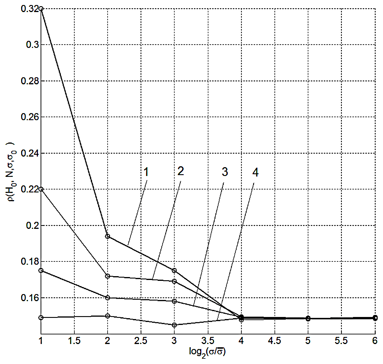
https://www.geosci-instrum-method-data-syst.net/8/209/2019/gi-8-209-2019-f03

Figure 3Results of calculation of the relative decrease factors for the errors: 1 – σ₀=0.5; 2 – σ₀=0.3; 3 – σ₀=0.1; 4 – σ₀=0.03.

Download

Analysis of the graphs shows that, for a fixed value σ, the introduced factor ρ decreases when σ₀ decreases, which is physically understandable. It is also seen that this factor tends to limit values with increasing σ. For a fixed H₀ , an increase in N leads to a decrease in the factor ρ. The performed statistical modelling for a wide range of parameters shows that the estimates for ρ are about 0.15–0.3, which indicates the efficiency of the proposed combined processing.

6 Conclusions

The proposed method for combined processing of the measurements of projections and absolute magnitudes of geomagnetic field intensity vectors and the corresponding two-stage algorithm developed appear to be satisfactorily workable. The testing of the developed combined processing algorithm on model and observatory measurement data proved its efficiency.

The approach realized in this paper, based on the proposed method, provides an increase in quality of the measurements of the projections of the geomagnetic intensity vector, allowing us to eliminate possible unwanted disturbances of artificial (anthropogenic) origin.

Statistical modelling for the developed algorithm for combined processing of measurements shows that at the first stage the relative decrease factor of RMS errors can reach values of 0.15–0.3, and at the second stage the decrease in the first-stage RMS errors can reach approximately 60 %–80 %.

Further reduction of the RMS noise errors can be implemented based on combined processing using local piecewise linear models for the values of projections and absolute magnitudes of geomagnetic field intensity vectors. The proposed combined processing algorithm can be implemented for many practically important tasks, in particular, when optimizing the operation of three-component accelerometer systems, three-component angular velocity sensors, or other three-component data arranged in a similar way. The technique allows for processing of the data with sampling intervals smaller than 1 s.

Code and data availability

The observatory geomagnetic data used for the tests in our study are available at the INTERMAGNET website (http://www.intermagnet.org; INTERMAGNET, 2018) as magnetograms or as digital data files.

Author contributions

VGG is the author and the main developer of the method presented in this research. Also, the basic work on programming was done by him. ADG performed the optimization and upgrade of the algorithm. RVS collected, analysed, and prepared the geomagnetic data for the computational tests.

Competing interests

The authors declare that they have no conflict of interest.

Acknowledgements

The results presented in this paper rely on data collected at the INTERMAGNET magnetic observatories. We thank the national institutes that support them and INTERMAGNET for promoting high standards of magnetic observatory practice (http://www.intermagnet.org).

We thank Igor M. Aleshin, as well as the anonymous reviewers, for their valuable comments that helped us to improve our article and clarify some significant details.

Financial support

This research has been supported by the Budgetary funding of the Geophysical Center of RAS, adopted by the Ministry of Science and Higher Education of the Russian Federation (grant no. 0145-2018-0002).

Review statement

This paper was edited by Luis Vazquez and reviewed by two anonymous referees.

References

Mandea, M. and Korte, M. (Eds.): Geomagnetic Observations and Models, Springer, -XV, 343 pp., available at: https://www.springer.com/gp/book/9789048198573 (last access: 3 August 2019), 2011.

Getmanov, V. G.: Nonlinear filtering of observations of a system of vector and scalar magnetometers, Meas. Tech.+, 56, 683–690, https://doi.org/10.1007/s11018-013-0265-3, 2013.

Getmanov, V. G., Sidorov, R. V., and Dabagyan, R. A.: The method of filtering signals using local models and weighted averaging functions, Meas. Tech.+, 58, 1029–1039, https://doi.org/10.1007/s11018-015-0837-5, 2015.

INTERMAGNET: International Real-Time Magnetic Observatory Network, available at: http://www.intermagnet.org/data-donnee/download-eng.php, last access: 27 April 2018.

Kramer, G.: Matematicheskie metody statistiki (Mathematical Methods of Statistics), Mir Publ., Moscow, Russia, 1975.

Merayo, J. M. G., Brauer, P., Primdahl, F., Petersen, J. R., and Nielsen, O. V.: Scalar calibration of vector magnetometers, Meas. Sci. Technol., 14, 120–132, 2000.

Olsen, N., Tøffner-Clausen, L., Sabaka, T. J., Brauer, P., Merayo, J. M. G., Jørgensen, J. L., Leger, J. M., Nielsen, O. V., Primdahl, F., and Risbo, T.: Calibration of the Ørsted vector magnetometer, Earth Planets Space, 55, 11–18, 2003.

Shakhtarin, B. I.: Fil'try Vinera i Kalmana (Wiener and Kalman filters), Gelios ARV Publ., Moscow, Russia, 2008.

Soborov, G. I., Skhomenko A. N., and Linko Y. R.: Sposob opredeleniya graduirovochnoy harakteristiki magnitometra (The method for determining the calibration characteristics of the magnetometer), Patent RF, no. 2481593, Federal Service for Intellectual Property of Russian Federation, Moscow, Russia, 2008.

Soloviev, A., Lesur, V., and Kudin, D.: On the feasibility of routine baseline improvement in processing of geomagnetic observatory data, Earth Planets Space, 70, 16, https://doi.org/10.1186/s40623-018-0786-8, 2018.