Advanced calibration of magnetometers on spin-stabilized   spacecraft based on parameter decoupling

Plaschke, Ferdinand; Auster, Hans-Ulrich; Fischer, David; Fornaçon, Karl-Heinz; Magnes, Werner; Richter, Ingo; Constantinescu, Dragos; Narita, Yasuhito

doi:https://doi.org/10.5194/gi-8-63-2019

Articles | Volume 8, issue 1

https://doi.org/10.5194/gi-8-63-2019

Articles | Volume 8, issue 1

Research article

12 Feb 2019

Research article |

| 12 Feb 2019

Advanced calibration of magnetometers on spin-stabilized spacecraft based on parameter decoupling

Ferdinand Plaschke, Hans-Ulrich Auster, David Fischer, Karl-Heinz Fornaçon, Werner Magnes, Ingo Richter, Dragos Constantinescu, and Yasuhito Narita

Abstract

Magnetometers are key instruments on board spacecraft that probe the plasma environments of planets and other solar system bodies. The linear conversion of raw magnetometer outputs to fully calibrated magnetic field measurements requires the accurate knowledge of 12 calibration parameters: six angles, three gain factors, and three offset values. The in-flight determination of 8 of those 12 parameters is enormously supported if the spacecraft is spin-stabilized, as an incorrect choice of those parameters will lead to systematic spin harmonic disturbances in the calibrated data. We show that published equations and algorithms for the determination of the eight spin-related parameters are far from optimal, as they do not take into account the physical behavior of science-grade magnetometers and the influence of a varying spacecraft attitude on the in-flight calibration process. Here, we address these issues. Based on decade-long developments and experience in calibration activities at the Braunschweig University of Technology, we introduce advanced calibration equations, parameters, and algorithms. With their help, it is possible to decouple different effects on the calibration parameters, originating from the spacecraft or the magnetometer itself. A key point of the algorithms is the bulk determination of parameters and associated uncertainties. The lowest uncertainties are expected under parameter-specific conditions. By application to THEMIS-C (Time History of Events and Macroscale Interactions during Substorms) magnetometer measurements, we show where these conditions are fulfilled along a highly elliptical orbit around Earth.

Download & links

Article (PDF, 2042 KB)

How to cite

How to cite.

Dates

Received: 24 Aug 2018 – Discussion started: 31 Aug 2018 – Revised: 30 Jan 2019 – Accepted: 06 Feb 2019 – Published: 12 Feb 2019

1 Introduction

The investigation of the plasma environment in the heliosphere, around planets, moons, comets, or other solar system bodies, requires accurate in situ observations of the magnetic field. Magnetometers on board spacecraft can provide these key measurements if accurately calibrated on the ground and in flight. The calibration process delivers the parameters needed to convert raw magnetometer measurements into magnetic field observations B=(B_x, B_y, B_z)^T in physically meaningful coordinate systems and units (usually nanotesla: nT). Commonly, a linear calibration equation is applied for this conversion (e.g., Fornaçon et al., 1999; Balogh et al., 2001 b; Auster et al., 2008):

\begin{matrix} (1) & B = C \cdot (B_{S} - O_{S}) . \end{matrix}

Here B_S=(B_S1, B_S2, B_S3)^T is the raw magnetometer output in non-orthogonal sensor coordinates, O_S corrects for non-vanishing magnetometers outputs in zero ambient fields (so-called offsets, which include spacecraft-generated magnetic fields at the sensor position), and C is the 3×3 coupling matrix. This matrix may have the following form (e.g., Kepko et al., 1996):

\begin{array}{l} C = & {(\begin{array}{ccc} \sin θ_{1} \cos ϕ_{1} & \sin θ_{1} \sin ϕ_{1} & \cos θ_{1} \\ \sin θ_{2} \cos ϕ_{2} & \sin θ_{2} \sin ϕ_{2} & \cos θ_{2} \\ \sin θ_{3} \cos ϕ_{3} & \sin θ_{3} \sin ϕ_{3} & \cos θ_{3} \end{array})}^{- 1} \\ (2) & \cdot (\begin{array}{ccc} G_{S 1} & 0 & 0 \\ 0 & G_{S 2} & 0 \\ 0 & 0 & G_{S 3} \end{array}) . \end{array}

The coupling matrix C depends on three scaling factors (G_S1, G_S2, and G_S3, also called the gains) and six angles (θ₁, θ₂, θ₃, and ϕ₁, ϕ₂, ϕ₃) which define the directions of the three sensor axes in the orthogonal coordinate system to which B pertains. Calibrating a magnetometer means finding the three gains, six angles, and three offset components (i.e., in total 12 parameters) so that B can accurately be obtained from B_S.

Ground calibration of magnetometers is facilitated by rotating them in Earth's magnetic field (Green, 1990). Similarly, operating a magnetometer on a spinning spacecraft, instead of on a three-axis stabilized spacecraft, enormously supports the in-flight determination of 8 of the 12 calibration parameters. These eight spin-related parameters are the two spin plane offset components, five of the six sensor direction angles (all but one defining the rotation about the spin axis), and the ratio of the spin plane gains. The reason is that an incorrect choice in any of those eight spin-related parameters leads to the appearance of clear, systematic signals at the spin frequency (also called the first harmonic) and/or at twice the spin frequency (second harmonic) in the de-spun magnetic field measurements. Hence, minimization of these signals can be used to determine the eight calibration parameters, as described in Farrell et al. (1995) and Kepko et al. (1996).

The other four (spin-unrelated) parameters are the absolute gains in the spin plane and along the spin axis, the spin axis offset, and the angle of rotation of the sensor about the spin axis. Gains and angle can be derived in flight through comparison of magnetic field measurements with the International Geomagnetic Reference Field (IGRF) or the Tsyganenko field models, which are fairly accurate close to Earth (e.g., Thébault et al., 2015; Tsyganenko and Sitnov, 2007). For the determination of the spin axis offset in flight, a list of different methods exists. Typically, the offset is obtained from careful analysis of Alfvénic magnetic field fluctuations, present in the pristine solar wind (e.g., Belcher, 1973; Hedgecock, 1975; Leinweber et al., 2008). If strongly compressional fluctuations are observed instead of Alfvénic fluctuations, then the mirror mode method may be used (Plaschke and Narita, 2016; Plaschke et al., 2017). The offset may also be obtained from comparison with measurements from an absolute magnetometer or time-of-flight measurements of electrons emitted and observed by an electron drift instrument (Georgescu et al., 2006; Nakamura et al., 2014; Plaschke et al., 2014). Furthermore, the spin axis offset may also be obtained in regions of space where the fields are known, for instance, in diamagnetic cavities in the vicinity of comets (Goetz et al., 2016 a, b).

From the preceding paragraphs, the reader might get the impression that in-flight calibration of magnetometers on spinning spacecraft is a solved issue, and in theory this is the case. However, as we will show in the following sections, the published methods for spin-aided calibration (Farrell et al., 1995; Kepko et al., 1996) are not optimal in practice because they do not take into account the physical behavior of the sensor package and the influence of a varying spacecraft attitude on the in-flight calibration.

This paper aims at identifying deficiencies and suggesting improvements with respect to the calibration equations (Eqs. 1 and 2) and the specific choice of the calibration parameters. Thereafter, we identify optimal conditions for spin-related calibration parameter determination. Finally, we introduce advanced algorithms for parameter determination based on our findings that facilitate the automation and distribution of calibration activities. A version of these algorithms is routinely applied to calibrate magnetometer data from the Magnetospheric Multiscale (MMS) mission (Burch et al., 2016; Torbert et al., 2016; Russell et al., 2016). The calibration principles and algorithms described here are based on developments at the Braunschweig University of Technology (Fornaçon et al., 2011) that have been successfully applied for decades to calibrate magnetometer data from, e.g., the Equator-S (Fornaçon et al., 1999), the Cluster (Balogh et al., 2001 a, b), and the Time History of Events and Macroscale Interactions during Substorms (THEMIS) missions (Angelopoulos, 2008; Auster et al., 2008).

2 Calibration equation and parameters

Equations (1) and (2) in principle allow for any linear conversion of B_S into B. The coupling matrix (Eq. 2) is obviously split into two components:

\begin{matrix} (3) & C = Θ \cdot G . \end{matrix}

Here, the diagonal matrix G only includes the gains, and the matrix Θ only includes the angular dependencies. Let us focus first on the matrix Θ. The parameters θ₁, θ₂, and θ₃ are the angles between the three mutually non-orthogonal sensor axes (directions S1–S3) and the spin axis in the z direction in an orthogonal, spin-axis-aligned, and spacecraft-fixed coordinate system (directions x, y, and z). The parameters ϕ₁, ϕ₂, and ϕ₃ correspond to the angles between the spacecraft-fixed x direction in the spin plane (x–y plane, perpendicular to the spin axis) and the projections of the sensor axes onto that plane. For simplicity, the sensor axes S1, S2, and S3 are assumed to be approximately aligned with x, y, and z. Note that all coordinate systems used in this paper are listed in Table 1.

Table 1List of coordinate system notations used in this paper similar to Table 1 in Kepko et al. (1996).

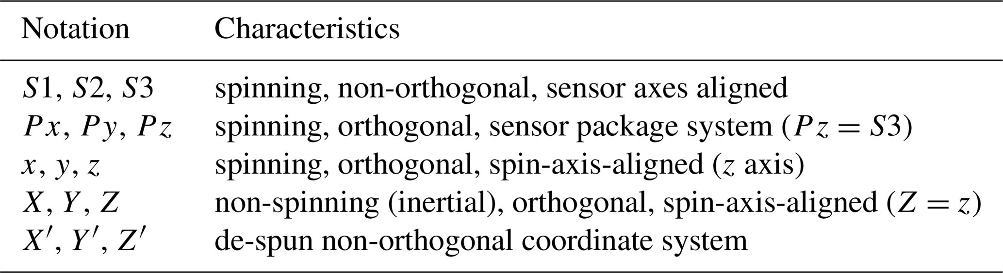
Download Print Version | Download XLSX

https://www.geosci-instrum-method-data-syst.net/8/63/2019/gi-8-63-2019-f01

Figure 1Sketch of the coordinate systems: (a) sensor axes in the sensor package coordinate system and (b) spin axis and rotation angles σ_Px and σ_Py in the sensor package coordinate system.

Download

The individual link of the sensor axes to a spacecraft-fixed, spin-axis-aligned system is an issue here as it does not reflect the actual situation on the spacecraft: there, the three sensor axes are typically packaged together into one sensor system. One of the design criteria of modern fluxgate magnetometer sensors is the temperature and long-term stability of the sensor axis directions as defined with respect to the sensor package. The angles between the sensor axes are usually well known from ground calibration activities (e.g., Auster et al., 2008; Russell et al., 2016), and we can expect the three angles between the sensor axes to be relatively stable parameters. Consequently, in a first step, the magnetometer output in non-orthogonal sensor coordinates should be transformed into an orthogonal sensor package fixed coordinate system (coordinates: Px, Py, Pz; see Table 1). The conversion matrix may have the following form:

\begin{matrix} (4) & Γ = {(\begin{array}{ccc} \sin θ_{S 1} & 0 & \cos θ_{S 1} \\ \cos ϕ_{S 12} \sin θ_{S 2} & \sin ϕ_{S 12} \sin θ_{S 2} & \cos θ_{S 2} \\ 0 & 0 & 1 \end{array})}^{- 1} . \end{matrix}

Here, θ_S1 and θ_S2 are the angles between the sensor axes S1 and S2 with respect to S3=Pz, and ϕ_S12 is the angle between the projections of S1 and S2 onto a plane perpendicular to S3, the Px–Py plane. Note that S1 lies in the Px–Pz plane (see Fig. 1a).

In the next step, the orientation of that sensor package system needs to be defined in a spacecraft-fixed spin-axis-aligned coordinate system. This latter transformation is expected to change every time there is a maneuver of the spacecraft, as fuel consumption will change the tensor of inertia and, thus, the spin axis direction in any spacecraft-fixed coordinate system. The spin axis direction can be defined in the orthogonal sensor package system using two parameters or angles. During maneuvers, only those two parameters or angles should change because the geometry inside the sensor package should not be affected. A rotation matrix Σ into a spin-axis-aligned coordinate system dependent on the two angles σ_Px and σ_Py can be defined as follows:

\begin{array}{l} Σ & = (\begin{array}{ccc} \cos σ_{P x} & 0 & - \sin σ_{P x} \\ 0 & 1 & 0 \\ \sin σ_{P x} & 0 & \cos σ_{P x} \end{array}) \\ (5) & \cdot (\begin{array}{ccc} 1 & 0 & 0 \\ 0 & \cos σ_{P y} & - \sin σ_{P y} \\ 0 & \sin σ_{P y} & \cos σ_{P y} \end{array}) . \end{array}

Here, σ_Py is the angle between Pz and the projection of the spin axis onto the Py–Pz plane, positive towards Py; σ_Px is the angle between that projection and the spin axis, positive towards Px. The angles are illustrated in Fig. 1b. Note that the spin axis is assumed to be approximately aligned with the Pz=S3 axis. As a result, the angles σ_Px and σ_Py will be small and can be associated with the Px and Py coordinates of a unit vector that points in spin axis direction.

Using the angles σ_Px and σ_Py to define the spin axis direction is advantageous over using the angles θ₃ and ϕ₃, as the latter angle is badly defined if θ₃ is small. Furthermore, it should also be noted that a change in direction of the spin axis requires an update of all angles of matrix Θ as defined above, even though the magnetometer (sensor) itself is unaffected. Only two parameters (σ_Px and σ_Py) need to be changed here to adapt the matrix Σ to the new spin axis direction.

To completely orient the sensor package (system) in the spin-axis-aligned coordinate system, a rotation about the spin axis (rotation matrix Φ) also needs to be taken into account:

\begin{matrix} (6) & Φ = (\begin{array}{ccc} \cos ϕ_{a} & - \sin ϕ_{a} & 0 \\ \sin ϕ_{a} & \cos ϕ_{a} & 0 \\ 0 & 0 & 1 \end{array}) . \end{matrix}

As we will show later, this rotation does not affect the spin tone content in the de-spun magnetic field observations. The angle is affected by the orientation of a magnetometer boom and may change due to boom bending (Farrell et al., 1995).

Altogether, we can replace the orthogonalization and reorientation matrix Θ by $Φ \cdot Σ \cdot Γ$ in Eq. (3). Let us focus then again on the gain matrix G in that equation. As mentioned in the Introduction, the spacecraft spin aids the determination of the ratio $g^{2} = G_{S 1} / G_{S 2}$ of the spin plane gains but not the absolute gains in the spin plane $G_{p} = \sqrt{G_{S 1} G_{S 2}}$ and along the spin axis G_a=G_S3. Hence, it makes sense to use the parameters g and G_p instead of G_S1 and G_S2 in the matrix G to decouple parameters that can be frequently updated from parameters that are only obtainable in flight from comparison to model fields or measurements of other instruments:

\begin{matrix} (7) & G = (\begin{array}{ccc} g G_{p} & 0 & 0 \\ 0 & G_{p} / g & 0 \\ 0 & 0 & G_{a} \end{array}) . \end{matrix}

Note that Kepko et al. (1996) use the difference of the inverse gains $Δ G_{21} = 1 / G_{S 2} - 1 / G_{S 1}$ instead of g. However, later changes in the absolute gains G_S1 and G_S2 then necessarily require an update of ΔG₂₁ in order to avoid perturbations at the second harmonic in the de-spun data. The gain ratio g, instead, is decoupled from changes in the absolute gains G_p and G_a.

The gains should be stable parameters in the absence of temperature variations. These variations in the gains can be determined from ground calibration, resulting in a diagonal gain correction matrix G_T(T_s, T_e) that is dependent on the magnetometer sensor (T_s) and electronics (T_e) temperatures. That matrix should be directly applied to the magnetometer output B_S, requiring the knowledge of the sensor and electronics temperatures:

\begin{matrix} (8) & B_{ST} = G_{T} (T_{s}, T_{e}) \cdot B_{S} . \end{matrix}

The resulting temperature-corrected output B_ST may then be further converted to B via the coupling matrix $C = Φ \cdot Σ \cdot Γ \cdot G$ and the offset vector O using Eq. (1), after replacing B_S with B_ST. This also has the advantage that the further applied absolute gains G_p and G_a and the gain ratio g² should all be approximately 1 and unitless.

Altogether, we suggest using the following improved calibration equation:

\begin{matrix} (9) & B = Φ \cdot Σ \cdot Γ \cdot G \cdot (\underset{= B_{ST}}{\underset{︸}{G_{T} (T_{s}, T_{e}) \cdot B_{S}}} - O_{S}), \end{matrix}

with matrices defined in Eqs. (4) to (7) instead of the simpler Eqs. (1) and (2). The parameters whose determination is supported by the spacecraft spin are θ_S1, θ_S2, ϕ_S12, σ_Px, σ_Py, g, O_S1, and O_S2.

3 Calibration parameter influence on spin tone harmonics

To determine the influence of the calibration parameters on the spin tone harmonic disturbances in the de-spun magnetic field measurements, we use a similar mathematical approach to Kepko et al. (1996) in this section. Based on the results, we go on to derive the optimal conditions for the determination of each parameter in Sect. 4.

First, we compute the temperature-corrected sensor output B_ST as a function of the external field B in the spinning coordinate system:

\begin{matrix} (10) & B_{ST} = G^{- 1} \cdot Γ^{- 1} \cdot Σ^{- 1} \cdot Φ^{- 1} \cdot B + O_{S} . \end{matrix}

We linearize all the matrices, using the following simplifying assumptions. The validity of these assumptions and the admissible deviations are discussed in Sect. 7.

\begin{array}{l} (11) & g \approx 1, G_{p} \approx 1, G_{a} \approx 1 \\ (12) & σ_{P x} \approx 0, σ_{P y} \approx 0 \\ (13) & θ_{S 1} \approx π / 2, δ θ_{S 1} = θ_{S 1} - π / 2 \approx 0 \\ (14) & θ_{S 2} \approx π / 2, δ θ_{S 2} = θ_{S 2} - π / 2 \approx 0 \\ (15) & ϕ_{S 12} \approx π / 2, δ ϕ_{12} = ϕ_{S 12} - π / 2 \approx 0 \end{array}

Furthermore, we assume ϕ_a≈0 without loss of generality. Dropping second-order factors, we obtain the following linearized inverted matrices used in Eq. (10):

\begin{array}{l} (16) & G^{- 1} = (\begin{array}{ccc} 1 / (g G_{p}) & 0 & 0 \\ 0 & g / G_{p} & 0 \\ 0 & 0 & 1 / G_{a} \end{array}) \\ (17) & Γ^{- 1} = (\begin{array}{ccc} 1 & 0 & - δ θ_{S 1} \\ - δ ϕ_{S 12} & 1 & - δ θ_{S 2} \\ 0 & 0 & 1 \end{array}) \\ (18) & Σ^{- 1} = (\begin{array}{ccc} 1 & 0 & σ_{P x} \\ 0 & 1 & σ_{P y} \\ - σ_{P x} & - σ_{P y} & 1 \end{array}) \\ (19) & Φ^{- 1} = (\begin{array}{ccc} 1 & ϕ_{a} & 0 \\ - ϕ_{a} & 1 & 0 \\ 0 & 0 & 1 \end{array}) . \end{array}

Furthermore, without loss of generality, we assume the magnetic field in the de-spun (inertial) coordinate system (directions X, Y, and Z) to be in the X–Z plane, and the spacecraft to spin around the Z axis, which corresponds to the z axis in the spacecraft-fixed, spin-aligned coordinate system (see Table 1). In that latter system, the field rotates and has the following form:

\begin{array}{l} (20) & B_{x} = B_{p} \cos ω t = B_{X} \cos ω t \\ (21) & B_{y} = B_{p} \sin ω t = B_{X} \sin ω t \\ (22) & B_{z} = B_{a} = B_{Z} . \end{array}

Here, ω is the angular frequency of the spacecraft rotation, usually determined from sun sensor or star tracker measurements, and t denotes the time. Inserting these relations in Eq. (10) yields the expected temperature-corrected output of the magnetometer in sensor coordinates. By applying the de-spun rotation matrix

\begin{matrix} (23) & D = (\begin{array}{ccc} \cos ω t & - \sin ω t & 0 \\ \sin ω t & \cos ω t & 0 \\ 0 & 0 & 1 \end{array}) \end{matrix}

to Eq. (10) to transform B_ST into a non-orthogonal, de-spun coordinate system (directions X^′, Y^′, and Z^′; see Table 1), after sorting by frequency and phase of the terms, and further dropping second-order factors, we obtain the following relations. They are structurally similar to Eqs. (11a)–(11c) in Kepko et al. (1996), but different in detail:

\begin{array}{l} B_{X^{'}} & = \frac{B_{p} (1 + g^{2})}{2 g G_{p}} \\ + \cos ω t [O_{S 1} + \frac{B_{a} (σ_{P x} - δ θ_{S 1})}{g G_{p}}] \\ - \sin ω t [O_{S 2} + \frac{g B_{a} (σ_{P y} - δ θ_{S 2})}{G_{p}}] \\ + \cos 2 ω t [\frac{B_{p} (1 - g^{2})}{2 g G_{p}}] \\ (24) & + \sin 2 ω t \frac{B_{p}}{2 G_{p}} [g ϕ_{a} - \frac{ϕ_{a}}{g} + g δ ϕ_{S 12}] \end{array}

\begin{array}{l} B_{Y^{'}} & = - \frac{B_{p}}{2 G_{p}} [\frac{1 + g^{2}}{g} ϕ_{a} + g δ ϕ_{S 12}] \\ + \cos ω t [O_{S 2} + \frac{g B_{a} (σ_{P y} - δ θ_{S 2})}{G_{p}}] \\ + \sin ω t [O_{S 1} + \frac{B_{a} (σ_{P x} - δ θ_{S 1})}{g G_{p}}] \\ - \cos 2 ω t \frac{B_{p}}{2 G_{p}} [g ϕ_{a} - \frac{ϕ_{a}}{g} + g δ ϕ_{S 12}] \\ (25) & + \sin 2 ω t [\frac{B_{p} (1 - g^{2})}{2 g G_{p}}] \end{array}

\begin{array}{l} B_{Z^{'}} & = \frac{B_{a}}{G_{a}} + O_{S 3} \\ - \cos ω t \frac{B_{p} σ_{P x}}{G_{a}} \\ (26) & + \sin ω t \frac{B_{p} σ_{P y}}{G_{a}} . \end{array}

These equations show how the parameters affect the signal content at the spin tone harmonics in the de-spun measurements. The first terms in all three Eqs. (24)–(26) are the primary measurements terms. In the spin plane, the ambient magnetic field only has a B_X=B_p component. Consequently, the first term of $B_{X^{'}}$ is approximately B_p, while the first term of $B_{Y^{'}}$ is approximately 0 as ϕ_a≈0 and δϕ_S12≈0. In the spin axis, we find $B_{Z^{'}} \approx B_{a}$ with G_a≈1 and O_S3≈0. In addition, superposed first and second harmonic signals are expected as functions of the calibration parameters. The first harmonic signals are described by the second and third terms in Eqs. (24)–(26). In the spin plane, Eqs. (24) and (25), the spin tone signals are the result of spin plane offsets O_S1∕2 and projections of the spin axis field B_a onto the spin plane. In the spin axis, Eq. (26), first harmonic disturbances are due to the projection of spin plane fields onto the spin axis, the reason being an incorrect description of the spin axis direction by the angles σ_Px∕y. Second harmonic signals are only expected in the de-spun spin plane components (fourth and fifth terms of Eqs. 24 and 25). These are due to a mismatch in spin plane gains (parameter g) or an unaccounted non-orthogonality between the spin plane sensor axes S1 and S2 (parameter δϕ_S12).

4 Favorable conditions for the determination of the calibration parameters

From the factors pertaining to the first and second harmonic terms of $B_{X^{'}}$ , $B_{Y^{'}}$ , and $B_{Z^{'}}$ (Eqs. 24 to 26), it is possible to derive the conditions that should be favorable for the determination of the eight previously mentioned parameters. These factors are

\begin{array}{l} (27) & [O_{S 1} + \frac{B_{a} (σ_{P x} - δ θ_{S 1})}{g G_{p}}] and [O_{S 2} + \frac{g B_{a} (σ_{P y} - δ θ_{S 2})}{G_{p}}] \\ (28) & [\frac{B_{p} σ_{P x}}{G_{a}}] and [\frac{B_{p} σ_{P y}}{G_{a}}] \\ (29) & [\frac{B_{p} (1 - g^{2})}{2 g G_{p}}] and \frac{B_{p}}{2 G_{p}} [g ϕ_{a} - \frac{ϕ_{a}}{g} + g δ ϕ_{S 12}] . \end{array}

Here, Eqs. (27) and (28) pertain to the spin tone disturbances in the de-spun spin plane and spin axis components, respectively, and Eq. (29) pertains to the second harmonic frequency disturbance (double spin tone frequency) in the spin plane components.

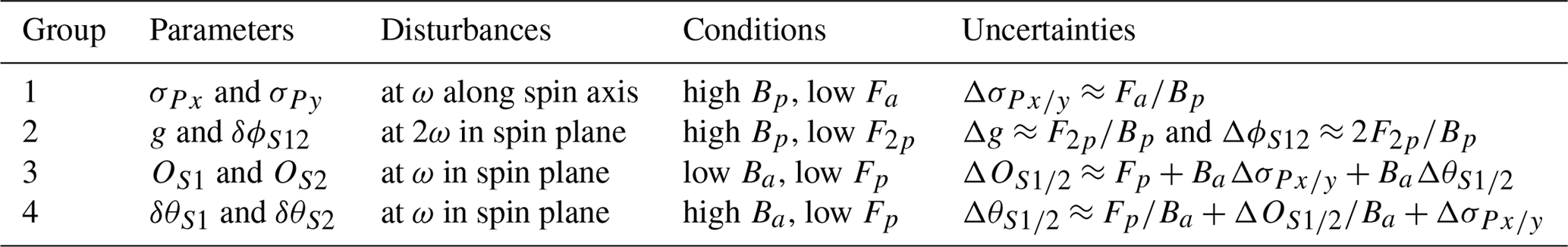
Table 2Parameters and favorable conditions.

Download Print Version | Download XLSX

As can be seen, the first factor of the latter group (Eq. 29) is dependent on B_p, the external field in the spin plane which we assume to be constant, on G_p, the absolute gain factor in the spin plane which should be approximately 1, and on $1 / g - g$ , which is 0 only if g=1. Hence, the presence of one part of the second harmonic disturbance, though modulated by B_p, is ultimately only dependent on g, the ratio of spin plane gains. Consequently, this relation can be used to determine g correctly. The signal to do that, in particular, the signal-to-noise ratio (SNR), is larger if B_p is larger. We capture this relation in the second line of Table 2. As the second harmonic disturbance in the spin plane is to be minimized to get g, the natural fluctuations around that frequency (of amplitude F_2p) should also be low in the spin plane. The uncertainty in g is then expected to be on the order of F_2p∕B_p.

The same is true for the complementary factor, on the right side of Eq. (29): this second harmonic disturbance is also modulated by B_p. When g is accurately determined, then the ϕ_a influence vanishes, and the entire factor can only vanish by correctly choosing δϕ_S12. Hence, to determine this parameter accurately, B_p should also be large and the natural fluctuations at the second harmonic should be of low amplitude (low F_2p). The uncertainty Δϕ_S12 of δϕ_S12 and, ultimately, ϕ_S12 is expected to be on the order of 2F_2p∕B_p (see line 2 in Table 2).

Let us focus on Eq. (28). The spin frequency disturbance is clearly modulated by B_p, as G_a should be close to 1, so B_p benefits the SNR. These disturbances vanish if σ_Px and σ_Py become 0, i.e., if they are precisely determined. A low amplitude in the natural fluctuations at the spin frequency along the spin axis F_a would also support the determination. The uncertainty in σ_Px and σ_Py is then expected to be on the order of $Δ σ_{P x / y} \approx F_{a} / B_{p}$ (line 1 in Table 2).

The first set of factors in Eq. (27) pertain to the spin frequency disturbances in the spin plane components. They consist of two parts: a spin plane offset component O_S1 or O_S2 and a term that is modulated by B_a and which may vanish if the difference (σ_Px−δθ_S1) or (σ_Py−δθ_S2) vanishes. Obviously, if B_a vanishes, then the spin plane spin frequency disturbances can only come from the spin plane offset components. Hence, for their determination, it is beneficial if the spin axis field B_a is low and if the natural fluctuation level around the spin frequency in the spin plane F_p is low. The uncertainty in O_S1 and O_S2 is then expected to be on the order of $F_{p} + B_{a} Δ σ_{P x / y} + B_{a} Δ θ_{S 1 / 2}$ (see line 3 of Table 2).

The remaining elevation angles δθ_S1 and δθ_S2 are most difficult to determine: it is beneficial if the spin axis field B_a is high. In addition, however, it is necessary that the spin axis itself is determined well, as the parameters σ_Px and σ_Py equally influence the spin tone signal in the spin plane as δθ_S1 and δθ_S2. Note that σ_Px and σ_Py can be independently determined by minimizing the spin frequency disturbances in the spin axis component. F_p should again be low. Altogether, the uncertainty in δθ_S1∕2 is on the order of $Δ θ_{S 1 / 2} \approx F_{p} / B_{a} + Δ O_{S 1 / 2} / B_{a} + Δ σ_{P x / y}$ (see line 4 of Table 2).

5 Parameter determination

Based on the findings from the previous section, we propose algorithms to determine the eight spin-related parameters in an iterative manner (Sect. 5.2 to 5.5). The algorithms are based on computing estimates of the parameters for short intervals and evaluate the uncertainties of those estimates based on the uncertainties indicated in Table 2. Then, the estimates with uncertainties below a certain acceptable threshold are chosen to form the basis of one parameter correction.

5.1 Precalibration

The temperature-dependent gains G_T(T_s, T_e) determined on the ground should be used to convert the raw magnetometer output B_S to a precalibrated, temperature-corrected intermediate product B_ST, according to Eq. (8).

The offset vector O_S and the calibration matrices Φ, Σ, Γ, and G should be initiated with the best known values at the time of calibration. At the beginning, these will be ground-obtained values:

for θ_S1, θ_S2, ϕ_S12, and O_S from ground magnetometer calibration,
for ϕ_a from nominal spacecraft design or mirror- and laser-based alignment measurements,
for σ_Px and σ_Py from an initial estimate of the spin axis direction (alternatively $σ_{P x} = σ_{P y} = 0$ may be chosen),
and $G_{p} = G_{a} = g = 1$ due to precalibration.

If in-flight calibration has already taken place, then these values will be superseded by better in-flight determined values.

5.2 Calibration of the spin axis direction

The entire interval of magnetic field measurements should be divided into small (overlapping) subintervals of length $t_{int} = 2 π n / ω$ , with n∈ℕ. The factor n should not be too small; hence, the subintervals should contain a number of spin periods, so that the spin tone at the spin frequency and also the power around that frequency can be accurately determined. On the other hand, subintervals should not be too large, so that the field or environmental conditions can be assumed constant.

For each of the subintervals, the uncertainties $Δ σ_{P x / y} \approx F_{a} / B_{p}$ need to be calculated (line 1 in Table 2). Conservatively, we choose B_p to be the minimal modulus of the spin plane field over the subinterval: $\min (\sqrt{B_{x}^{2} + B_{y}^{2}})$ . F_a can be estimated by taking the maximum of the discrete Fourier components F_a± of the spin axis magnetic field B_z at frequencies ω_± that are slightly over and under the spin frequency: $ω_{\pm} = 2 π n_{\pm} / t_{int}$ , with $n_{\pm} \in N$ and slightly over and under n:

\begin{array}{l} (30) & F_{a \pm} = F (B_{z}, ω_{\pm}) = |\frac{2}{N} \sum_{k = 0}^{N - 1} B_{z} (t_{0} + k δ t) \exp (- i ω_{\pm} k δ t)| \\ (31) & F_{a} = \max (F_{a \pm}) . \end{array}

Here t₀ is the start of a subinterval considered, N is the number of magnetic field measurement samples in that subinterval, and δt is the sampling period. The frequencies ω₊ and ω₋ should sufficiently differ from ω to avoid leakage from spin tone. However, ω₊ and ω₋ should also be close enough to ω so that the amplitudes at those frequencies resemble the natural amplitude level at the spin frequency. Note that the optimal choice of ω₊ and ω₋ is subinterval-specific. In practice, however, fixed frequencies can be used that are at some distance $| ω_{\pm}$ –ω|, if that distance is safely larger than usual spin tone spectral peak widths.

From here on, we use ℱ(B, ω) to denote the Fourier component of B at frequency ω. It should be noted that it may be recommended to de-trend the B data before computing ℱ(B, ω), by simply subtracting a linear fit. Linear trends will not occur if the external field can be assumed to be constant. In many real applications, however, the spacecraft will move through field gradients during subintervals considered, and, in these cases, the linear trend in the field measurements will increase the spectral content across the spectrum.

Parameter estimates σ_Px and σ_Py are determined by minimization of the spin tone S_a in the spin axis component: S_a=ℱ(B_z, ω). This minimization is performed for each subinterval. Hence, we obtain for each subinterval one estimate for σ_Px, for σ_Py, and for the uncertainty Δσ_Px∕y. A final parameter update for σ_Px and σ_Py for the entire interval of interest may be obtained by selecting the most accurate subinterval estimates of those parameters, pertaining to minimal uncertainties Δσ_Px∕y. From those estimates, the median or average may be computed. The selection of the best estimates can be threshold-based with respect to Δσ_Px∕y.

5.3 Calibration of gain ratio and azimuthal angle

As detailed in the previous section, Sect. 5.2, an interval of interest is divided into short (overlapping) subintervals of length $t_{int} = 2 π n / ω$ . For each of these subintervals, the uncertainties Δg and Δϕ_S12 are computed (see line 2 in Table 2). Therefore, the fluctuation amplitudes $F_{2 p} = \max (F (\sqrt{B_{x}^{2} + B_{y}^{2}}$ , 2ω_±)) need to be computed, with $2 ω_{\pm} = 4 π n_{\pm} / t_{int}$ and $n_{\pm} \in N$ slightly over and under n. Subsequently, the parameters g and δϕ_S12 are determined for each subinterval by minimization of $S_{2 p} = F (\sqrt{B_{x}^{2} + B_{y}^{2}}$ , 2ω). From the set of g and δϕ_S12 estimates from all subintervals, those associated with the lowest uncertainties can be chosen to yield final updates for g and δϕ_S12.

It should be noted that we are using here the modulus of the spin plane field ( $\sqrt{B_{x}^{2} + B_{y}^{2}} = \sqrt{B_{X}^{2} + B_{Y}^{2}}$ ) to compute F_2p and S_2p instead of any individual spin plane component (B_X or B_Y) in a de-spun coordinate system, as would be suggested by the analytical treatment outlined in Sect. 3. Both approaches (using the modulus or a de-spun component) are, however, mathematically equivalent. To show this, we can compute $\sqrt{B_{X^{'}}^{2} + B_{Y^{'}}^{2}}$ using Eqs. (24) and (25). From the sum $B_{X^{'}}^{2} + B_{Y^{'}}^{2}$ , only those terms are large which contain the first term of Eq. (24) because all other terms are products of multiple small factors and, hence, can be omitted due to linearization. Taking that into account, we obtain $\sqrt{B_{X^{'}}^{2} + B_{Y^{'}}^{2}} \approx B_{X^{'}}$ . Hence, $\sqrt{B_{x}^{2} + B_{y}^{2}}$ contains the field and variations corresponding to the de-spun component, along which the external field is pointing. Evaluating $\sqrt{B_{x}^{2} + B_{y}^{2}}$ is hence equivalent to evaluating B_X if the field points in the X direction. This result is based on the assumption of the spin tone and second harmonic terms being small in comparison to the constant spin plane magnetic field, which should be fulfilled even in low field conditions if the initial set of calibration parameters is not too inaccurate. Note also that it is not possible to obtain additional information with respect to the calibration parameters by evaluating the field-perpendicular component B_Y because the coefficients pertaining to the sin and cos terms of $B_{X^{'}}$ and $B_{Y^{'}}$ are the same (compare Eqs. 24 and 25).

The equivalence of the approaches (using the modulus or a de-spun component) brings up two questions: (i) why did we not use the modulus when calculating the influences of the spin-related parameters in Sect. 3 and (ii) why would we prefer using the modulus over a de-spun component here and in any practical application of the calibration algorithms outlined in this Sect. 5? The answer to question (i) is that the mathematical treatment of the modulus is slightly more involved than the treatment of the individual de-spun coordinates. Furthermore, Sect. 3 follows the approach of Kepko et al. (1996), who also use de-spun coordinates. Therefore, our results from Sect. 3 become directly comparable to the results of their study. In their and our analytical treatments, the de-spinning process is exactly defined, perfectly known, and accurate. Hence, it does not introduce additional uncertainty into the calibration process. This latter statement is not true in any real application, which leads us to the answer of question (ii): the modulus of the spin plane field is readily available in any spinning coordinate system. De-spinning is not necessary for magnetometer calibration, and it is not advised because it could introduce additional, unnecessary uncertainty.

5.4 Calibration of spin plane offsets

The uncertainties for each subinterval are computed as suggested in line 3 of Table 2. Therefore, the maximum of the spin axis field ( $B_{a} = \max | B_{z} |$ ) over each subinterval should be used. F_p is evaluated following Eq. (31). Furthermore, estimates for the uncertainties Δσ_Px∕y and Δθ_S1∕2 need to be obtained. These may be based on the variability of the selected estimates of σ_Px∕y (see Sect. 5.2) and δθ_S1∕2 (see Sect. 5.5) used to compute the final values of those parameters.

The offset estimates O_S1 and O_S2 are determined for each subinterval by minimization of $S_{p} = F (\sqrt{B_{x}^{2} + B_{y}^{2}}$ , ω). From the set of O_S1 and O_S2 estimates, the most accurate can be chosen to compute final updates for the spin plane offsets. It should be noted that the offsets are known to be the most variable parameters. Hence, it could be desirable to compute final offset updates more often than updates of other spin-related parameters, if possible.

5.5 Calibration of elevation angles

The uncertainties for each subinterval are computed as suggested in line 4 of Table 2, this time using $B_{a} = \min | B_{z} |$ . Estimates for the uncertainties Δσ_Px∕y and ΔO_S1∕2 need to be obtained, e.g., from the variability of selected σ_Px∕y and O_S1∕2 estimates. Subsequently, the elevation angles δθ_S1 and δθ_S2 are determined for each subinterval by minimization of $S_{p} = F (\sqrt{B_{x}^{2} + B_{y}^{2}}$ , ω). From the set of δθ_S1 and δθ_S2 estimates, the most accurate can be chosen (lowest uncertainties) to yield final updates of those parameters.

It should be noted that the same quantity S_p is minimized to obtain the elevation angles δθ_S1 and δθ_S2 and the offset components O_S1 and O_S2. Hence, the final selection of estimates according to the uncertainties Δθ_S1∕2 and ΔO_S1∕2, which are heavily dependent on $| B_{z} |$ , is very important here. In low $| B_{z} |$ , minimization of S_p yields the offset components, whereas in high fields the offsets do not matter any more and any spin tone may safely be attributed to an incorrect choice of the elevation angles if the spin axis direction is precisely known.

5.6 Exclusion of data intervals

Certain intervals may be excluded from parameter determination, as some of the underlying assumptions may not be met well. For instance, intervals featuring large spacecraft and sensor temperature changes should be avoided, as parameters may vary within such intervals. Hence, uncertainties in the parameters may be significantly higher than what is reflected in the uncertainty estimates stated in Table 2. Large temperature variations are expected during eclipse intervals, when the spacecraft is in shadow (e.g., of Earth), and hours after eclipse intervals as temperatures relax to stationary values. Furthermore, magnetic field measurements at saturation levels need to be avoided. Lastly, intervals during and after spacecraft maneuvers may be problematic for calibration, as the spin axis will fluctuate during maneuvers and nutation may be visible for periods of time after maneuvers. It should be noted that all these considerations are spacecraft- and orbit-specific.

6 Application to THEMIS data

To ascertain the accuracies that parameters may be determined with in different regions of near-Earth space, on a highly elliptical orbit around Earth, we apply the algorithms detailed above to two days (20 and 21 July 2007) of THEMIS-C (Angelopoulos, 2008) fluxgate magnetometer (FGM) data (Auster et al., 2008). The data are available at 4 Hz sampling frequency (data product: FGL); they are already fully calibrated and the applied calibration parameters do not change over the two days considered. The magnitudes of the magnetic field along the spin axis $| B_{z} |$ and in the spin plane $\sqrt{B_{x}^{2} + B_{y}^{2}}$ are displayed in Fig. 2a in red and blue, respectively.

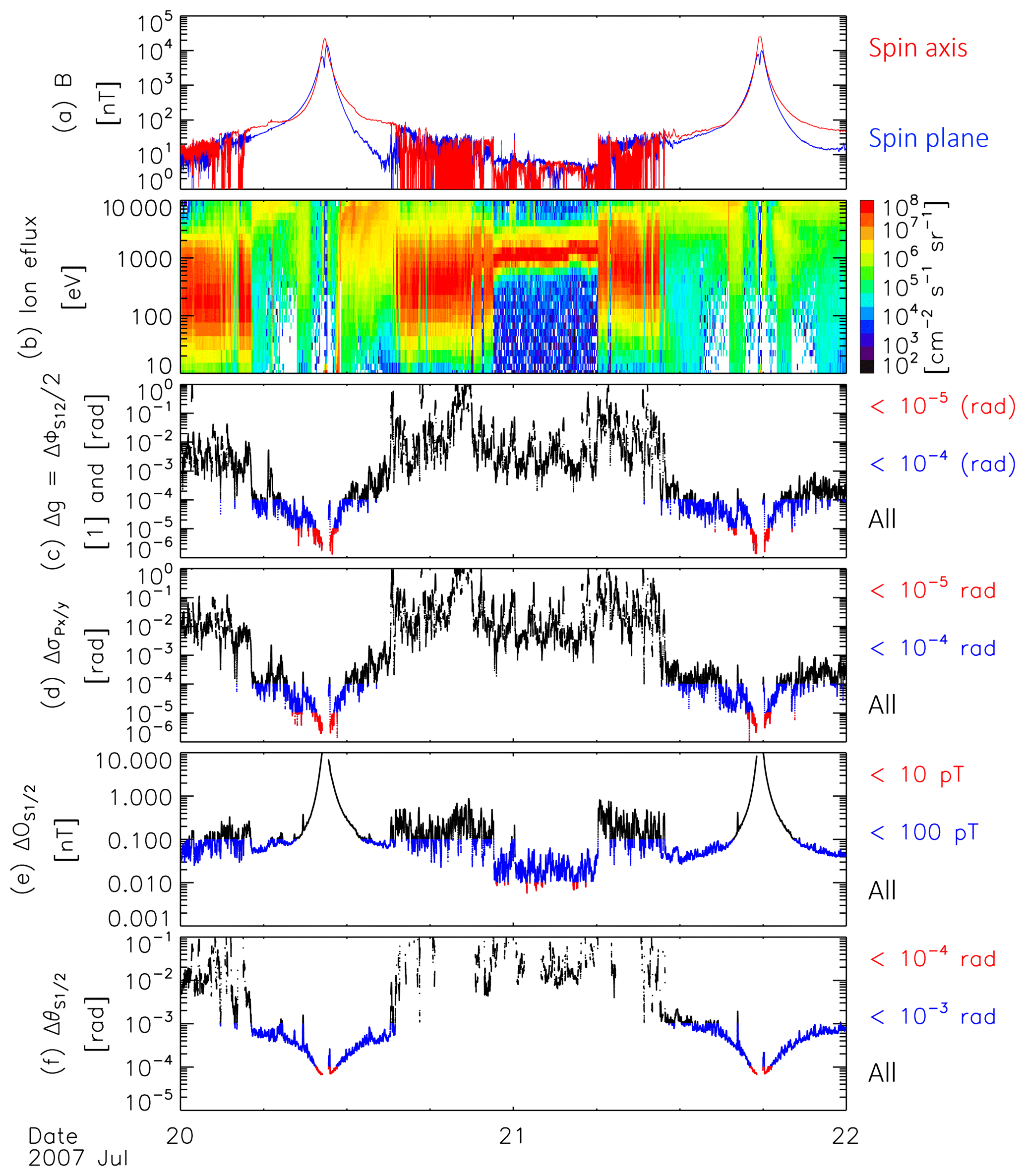
https://www.geosci-instrum-method-data-syst.net/8/63/2019/gi-8-63-2019-f02

Figure 2From top to bottom: (a) magnitude of the spin axis and spin plane magnetic fields in red and blue, (b) omnidirectional ion spectral energy flux densities, and (c–f) uncertainties of the estimates of the respective calibration parameters calculated in accordance with Table 2.

Download

The different regions that THEMIS-C went through during these two particular days are best identified using the omnidirectional ion spectral energy flux densities, measured by the electrostatic analyzer (ESA; McFadden et al., 2008) and displayed in Fig. 2b. At the beginning of 20 July 2007, THEMIC-C is located in the dayside magnetosheath. This is clearly visible in the broad ion energy spectrum, which is characteristic of the thermalized solar wind plasma population present downstream of the bow shock. THEMIS-C fully transitions through the magnetopause into the magnetosphere at about 05:06 UT, moving inbound towards perigee at about 10:27 UT. At about 15:33 UT, THEMIS-C went back into the magnetosheath until about 22:33 UT, when it transitioned through the bow shock into the solar wind, characterized by a narrow energy signature, corresponding to a cold plasma moving at solar wind speed. On 21 July, THEMIS-C went back into the magnetosheath at about 06:07 UT, and then went further into the magnetosphere at about 10:53 UT. The perigee pass on that day took place at about 17:47 UT.

As can be seen in Fig. 2a, the solar wind interval is characterized by low magnetic fields, typically below 10 nT. In the dayside magnetosheath, the field strength is somewhat higher, on the order of a few tens of nanotesla, and highly fluctuating. Inside the magnetosphere, the fluctuation level is again low. The lowest field strengths of a few tens of nanotesla are measured on the earthward side of the magnetopause, so just inside the inner magnetosphere. The field strength continuously increases towards Earth. On this particular THEMIS-C orbit, field strengths on the order of 10⁴ nT are reached along the spin axis and in the spin plane close to perigee. As discussed above, both the fluctuation levels and field strengths have a major influence on the expected uncertainties of the calibration parameter estimates. We determine the parameters and the corresponding uncertainties for overlapping subintervals of 100 spin periods each, a spin period lasting for approximately 3 s. Hence, the subintervals have interval lengths of approximately 5 min. Note that we do not consider subintervals containing fields above 2×10⁴ nT, due to FGM instrument saturation, and also excluded intervals in eclipse (Earth shadow) around perigee that lasted for approximately 22 min per orbit. Over the remaining times, temperature variations at the FGM sensor and electronics are limited to within 3^∘. In the THEMIS case, these small variations are not expected to have a significant influence on the calibration parameters.

Subinterval lengths of 100 spin periods ensure good estimates of the power at around (and double) the spin frequency $ω = 2 π / (3 s) \approx 2$ rad s⁻¹, while the calibration parameters to be determined and the ambient magnetic field conditions may well be considered constant over such short intervals. Estimates of the power F_a±, F_p±, and F_2p± around (double) the spin frequency are taken at 85 % and 115 % of ω and at 185 % and 215 % of ω, respectively. Following the equations from Table 2 and from Sect. 5.2 to 5.5 above, we determine the uncertainties for the calibration parameter estimates for all subintervals. They are shown in Fig. 2c–f.

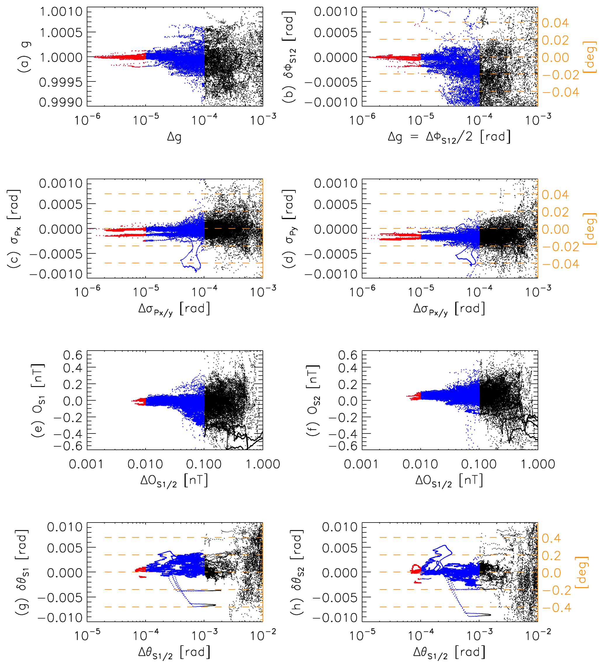
https://www.geosci-instrum-method-data-syst.net/8/63/2019/gi-8-63-2019-f03

Figure 3Calibration parameter estimates as a function of their respective uncertainties. Threshold levels for blue and red marked estimates are the same as in Fig. 2. Panels (b–d), (g), and (h) have secondary axes in orange, showing parameter values in degrees.

Download

Figure 2c and d show the uncertainties $Δ g = Δ ϕ_{S 12} / 2$ and Δσ_Px∕y. For the corresponding parameters, uncertainties on the order of 10⁻⁴ (rad) are generally acceptable. In the case of the gain ratio parameter g, an error of 10⁻⁴ would translate into an absolute error of 1 nT in 10 000 nT fields. With respect to the angle ϕ_S12 (or δϕ_S12) and to the spin axis angles σ_Px∕y, an error of $1 \times 10^{- 4}$ rad is equivalent to approximately 0.5 % of a degree. Uncertainties below 10⁻⁴ (rad) are marked in blue in Fig. 2c and d. As can be seen, estimates of g, ϕ_S12, and σ_Px∕y with uncertainties below this threshold can be obtained almost everywhere in the inner magnetosphere, where fields are relatively stable, but not in the magnetosheath (fluctuations too high) or in the solar wind (fields too low). Estimates associated with uncertainties below 10⁻⁵ (rad) are marked in red in Fig. 2c and d. These are only obtained in the regions of highest ambient fields, close to perigee.

The parameter estimates themselves (g, δϕ_S12, σ_Px, and σ_Py) are shown in Fig. 3a to d as a function of their respective uncertainties. Again, uncertainty thresholds of 10⁻⁴ and 10⁻⁵ (rad) are marked in blue and red, respectively. Taking the averages of the estimates associated with uncertainties below 10⁻⁵ (rad), we obtain

\begin{array}{l} (32) & 〈 g 〉 = 0.99998 \pm 0.00004 \\ (33) & 〈δ ϕ_{S 12}〉 = (- 3 \pm 6) \times 10^{- 5} rad \\ (34) & 〈σ_{P x}〉 = (- 7 \pm 6) \times 10^{- 5} rad \\ (35) & 〈σ_{P y}〉 = (- 1.7 \pm 0.4) \times 10^{- 4} rad . \end{array}

Here, the error values are the corresponding standard deviations of the estimates. We see that all parameters are close to 0 (or 1 in the case of g); an update may only be advised for σ_Py, as its deviation from 0 is significantly larger than the error value (see Fig. 3d).

In Fig. 3c and d, a split in values associated with low uncertainties can be clearly seen. A closer look at this phenomenon reveals that lower/higher σ_Px∕σ_Py values correspond to times before/after perigee passes. Hence, the spin axis direction in the orthogonalized sensor package coordinate system changes during perigee. This might be related to a temperature-driven change in spacecraft geometry, i.e., in boom alignment to the spacecraft body, occurring in eclipse during perigee passes.

In order to calculate the uncertainties of the offset and elevation angle estimates (ΔO_S1∕2 and Δθ_S1∕2; see lines 3 and 4 in Table 2), we have to assume uncertainties in the knowledge of the spin axis direction angles (Δσ_Px∕y), the offsets (ΔO_S1∕2), and the elevation angles (Δθ_S1∕2). Based on Eq. (35), we set $Δ σ_{P x / y} = 6 \times 10^{- 5}$ rad. Furthermore, as we can justify this a posteriori based on Eqs. (37) and (39), we set $Δ O_{S 1 / 2} = 25$ pT and $Δ θ_{S 1 / 2} = 7 \times 10^{- 4}$ rad. Therefore, we obtain the uncertainty estimates per subinterval shown in Fig. 2e and f.

The offsets directly influence the absolute accuracies of the magnetic field measurements. Typically, uncertainties on the order of or below 0.1 nT are desired in low fields. Uncertainties meeting this threshold are marked in blue in Fig. 2e. As can be seen, corresponding offset estimates can be routinely obtained in the solar wind, due to the low fields, and also in the outer, low field parts of the inner magnetosphere. Within the magnetosheath, however, many estimate uncertainties surpass the threshold as the fluctuations levels are too high for accurate offset determinations. Estimates with uncertainties below 10 pT (in red) can only be obtained in the solar wind at low fields. From those (red dots in Fig. 3e and f), we obtain average offsets of

\begin{array}{l} (36) & 〈O_{S 1}〉 = (- 0.007 \pm 0.023) nT \\ (37) & 〈O_{S 2}〉 = (0.036 \pm 0.025) nT . \end{array}

The error values here motivate the choice of ΔO_S1∕2 for the computation of the uncertainties of the elevation angles. These angles should also be known to the order of 10⁻⁴ rad. Unfortunately, estimates with uncertainties lower than this threshold are only obtained in very high fields, close to perigee, as can be seen by the red dots in Figs. 2f and 3g and h. The blue dots correspond to the lower threshold of 10⁻³ rad in this case, already equivalent to 5.7 % of a degree in angular uncertainty. From the δθ_S1∕2 estimates pertaining to uncertainties lower than 10⁻⁴ rad we obtain the following averages:

\begin{array}{l} (38) & 〈δ θ_{S 1}〉 = (5 \pm 4) \times 10^{- 4} rad \\ (39) & 〈δ θ_{S 2}〉 = (3 \pm 7) \times 10^{- 4} rad . \end{array}

Within the group of sensor orthogonalization angles (δθ_S1, δθ_S2, and δϕ_S12) and spin axis angles (σ_Px and σ_Py), these elevation angles are least accurately defined. Apparently, it is difficult to determine them to accuracies on the order of 10⁻⁴ rad or better. When determined on the ground, in higher fields, the parameters δθ_S1∕2 may however be better determined, with lower uncertainties than 10⁻⁴ rad. Hence, regular in-flight updating of these parameters may not be recommended, as those updates may introduce unnecessary jitter without any benefit for the overall accuracy of the magnetometer calibration.

7 Discussion on linearization assumptions

The only purpose of linearizing the calibration equation in Sect. 3 is to obtain the uncertainty relations shown in the right column of Table 2. These uncertainties (Δσ_Px∕y, Δg, Δϕ_S12, ΔO_S1∕2, and Δθ_S1∕2) are used to evaluate which calibration parameter estimates (from which subintervals) are most suitable to compute final calibration parameter updates. The estimates themselves are calculated using the nonlinearized calibration equation, Eq. (9). Hence, simplifications and assumptions associated with linearization do not influence the accuracy of those estimates. They only influence the accuracy of their uncertainties.

To obtain these uncertainties, a series of assumptions need to be made, e.g., in the form of Eqs. (11) to (15). This approach raises the question of how much the calibration parameters may be allowed to deviate from the assumed values. As shown in Sect. 6, we are interested in the orders of magnitude (factor of 10) of the uncertainties Δσ_Px∕y, Δg, Δϕ_S12, ΔO_S1∕2, and Δθ_S1∕2. Conservatively limiting the errors in these uncertainties to a factor of 2, and taking into account the multiplication of parameters due to Eq. (10), we can allocate lower limit individual admissible error factors of $\sqrt[4]{2} = 1.189$ to gain factors g, G_p, and G_a, as well as angles σ_Px, σ_Py, δθ_S1, δθ_S2, δϕ_S12, and ϕ_a. Such error factors of 1.189 or, equivalently, deviations by 19 % from the assumed values are extraordinarily large when compared to the accuracy in the knowledge of the calibration parameters and of the geometry of the sensor and spacecraft, even before performing any in-flight calibration. For the angles, this means that deviations from 0 by up to 11^∘ are acceptable (arcsin (19 %)); note that alignment uncertainties and deviations from sensor orthogonality should usually be lower than 1^∘. For the gains, deviations by 19 % would be acceptable; ground calibration, however, should reduce these deviations to less than 0.1 %. Hence, the assumptions made to linearize the calibration equation are not restrictive at all and can easily be fulfilled in practice.

8 Further discussion and conclusions

The orthogonalization angles are known to be relatively stable when compared to the spin axis direction angles. Fortunately, as shown in Sect. 6, the spin axis angles can be updated with high accuracy more regularly than the sensor elevation angles δθ_S1 and δθ_S2. The parameter decoupling introduced in Sect. 2 pays off here, as spin axis variations do not require redetermination of the sensor elevation angles as would be the case when using the calibration Eq. (1) with the coupling matrix (Eq. 2) instead of Eq. (9).

It should be noted that both Eqs. (1) and (9) assume raw magnetometer outputs to be linearly transformable into accurate magnetic field estimates. This assumption of linearity can only be fulfilled to a certain degree when dealing with actual magnetometer hardware. Nonlinearities (e.g., Auster et al., 2008; Russell et al., 2016) will adversely affect the calibration as described here if not characterized, quantified, and corrected beforehand, as they produce spin tone and higher harmonic signals in the magnetic field measurements. THEMIS FGM data, for instance, suffer from slight nonlinearities in digital-to-analogue converters that are part of the magnetometer hardware. These are known from ground characterization of the instruments and are routinely corrected in advance of any in-flight calibration activities and/or any conversion of magnetometer outputs into calibrated magnetic field measurements (Auster et al., 2008).

Assuming instrument linearity, the uncertainty-based approach to determining the spin-related calibration parameters allows for a meaningful estimation of the error alongside any parameter updates. These errors can be compared to the uncertainties of the already known parameters, determined either on the ground or in flight. Therewith, it is possible to decide whether any update of the calibration parameters is necessary or advised or, instead, would just introduce unnecessary variations in the calibration parameters over time.

In addition, the availability of calibration parameter estimates associated with low uncertainties, sufficient in number and quality, determines what is possible in terms of cadence of parameter updates. This availability depends on the orbit of the spacecraft (the presence in regions of certain field conditions) and also on the spin period of the spacecraft. In general, short spin periods (high spacecraft spin frequencies) are favorable, as they increase the number of spins that may be taken into account in subintervals of certain length. A larger number of spin periods reduces the influence of natural field fluctuations at (double) the spin frequency, while short subinterval lengths ensure the constancy of the parameters and environmental conditions. In the given THEMIS-C example, the spin plane offsets O_S1∕2 may be continuously tracked while the spacecraft remained in the solar wind and in the low field parts of the magnetosphere. The spin axis components σ_Px∕y, the gain ratio g, and azimuthal orthogonalization angle ϕ_S12 can easily be determined separately before and after each perigee pass, whereas accurate determinations of the elevation angles θ_S1∕2 may only be possible when taking into account estimates from several spacecraft orbits.

Finally we would like to note that the benefits of parameter decoupling (i.e., a sensible choice of parameters when taking into account the behavior of the magnetometer and spacecraft hardware) and of the uncertainty-based determination of those parameters are not tied to the exact definitions of the calibration equation (Eq. 9) and matrices (Eqs. 4 to 7). For example, the offsets may be applied in an orthogonal, spacecraft-fixed coordinate system instead of in the sensor coordinate system if the main contribution to the offsets is expected from spacecraft stray fields at the sensor position. The order of the gain, orthogonalization, and alignment matrices (here G, Γ, Σ, and Φ) may be changed, and/or the 12 degrees of freedom of the calibration parameters may be distributed over a larger number of matrices and offset vectors to account for changes pertaining to different parts of the magnetometer–spacecraft system in different coordinate systems (e.g., see equations in Fornaçon et al., 1999; Auster et al., 2008). Hence, while following the principles set out in this paper, a different set of calibration parameters and corresponding calibration equation may be specifically selected for each magnetometer–spacecraft combination.

Data availability

Data from the THEMIS mission including FGM and ESA data are publicly available from the University of California, Berkeley, and can be obtained from http://themis.ssl.berkeley.edu/data/themis (THEMIS, 2018).

Author contributions

FP, DF, and WM conceived the study. KHF, HUA, and IR contributed key knowledge and experience in spacecraft magnetometer calibration. DC and YN helped with the derivation and interpretation of equations.

Competing interests

The authors declare that they have no conflict of interest.

Acknowledgements

We acknowledge NASA contract NAS5-02099 and Vassilis Angelopoulos for use of data from the THEMIS mission. Specifically, we acknowledge Charles W. Carlson and James P. McFadden for use of ESA data and Karl-Heinz Glassmeier, Hans-Ulrich Auster, and Wolfgang Baumjohann for the use of FGM data provided under the lead of the Technical University of Braunschweig and with financial support from the German Ministry for Economy and Technology and the German Center for Aviation and Space (DLR) under contract 50 OC 0302.

Edited by: Valery Korepanov
Reviewed by: two anonymous referees

References

Angelopoulos, V.: The THEMIS Mission, Space Sci. Rev., 141, 5–34, https://doi.org/10.1007/s11214-008-9336-1, 2008. a, b

Auster, H. U., Glassmeier, K. H., Magnes, W., Aydogar, O., Baumjohann, W., Constantinescu, D., Fischer, D., Fornaçon, K. H., Georgescu, E., Harvey, P., Hillenmaier, O., Kroth, R., Ludlam, M., Narita, Y., Nakamura, R., Okrafka, K., Plaschke, F., Richter, I., Schwarzl, H., Stoll, B., Valavanoglou, A., and Wiedemann, M.: The THEMIS Fluxgate Magnetometer, Space Sci. Rev., 141, 235–264, https://doi.org/10.1007/s11214-008-9365-9, 2008. a, b, c, d, e, f, g

Balogh, A., Cargill, P. J., Carr, C. M., Dunlop, M. W., Horbury, T. S., Lucek, E. A., and Cluster FGM Investigator Team: Magnetic Field Observations on Cluster: an Overview of the First Results, in: Sheffield Space Plasma Meeting: Multipoint Measurements versus Theory, vol. 492 of ESA Special Publication, edited by: Warmbein, B., European Space Agency, Noordwijk, the Netherlands, p. 11, 2001a. a

Balogh, A., Carr, C. M., Acuña, M. H., Dunlop, M. W., Beek, T. J., Brown, P., Fornaçon, K.-H., Georgescu, E., Glassmeier, K.-H., Harris, J., Musmann, G., Oddy, T., and Schwingenschuh, K.: The Cluster Magnetic Field Investigation: overview of in-flight performance and initial results, Ann. Geophys., 19, 1207–1217, https://doi.org/10.5194/angeo-19-1207-2001, 2001b. a, b

Belcher, J. W.: A variation of the Davis–Smith method for in-flight determination of spacecraft magnetic fields, J. Geophys. Res., 78, 6480–6490, https://doi.org/10.1029/JA078i028p06480, 1973. a

Burch, J. L., Moore, T. E., Torbert, R. B., and Giles, B. L.: Magnetospheric Multiscale Overview and Science Objectives, Space Sci. Rev., 199, 5–21, https://doi.org/10.1007/s11214-015-0164-9, 2016. a

Farrell, W. M., Thompson, R. F., Lepping, R. P., and Byrnes, J. B.: A method of calibrating magnetometers on a spinning spacecraft, IEEE T. Magnet., 31, 966–972, https://doi.org/10.1109/20.364770, 1995. a, b, c

Fornaçon, K.-H., Auster, H. U., Georgescu, E., Baumjohann, W., Glassmeier, K.-H., Haerendel, G., Rustenbach, J., and Dunlop, M.: The magnetic field experiment onboard Equator-S and its scientific possibilities, Ann. Geophys., 17, 1521–1527, https://doi.org/10.1007/s00585-999-1521-3, 1999. a, b, c

Fornaçon, K.-H., Georgescu, E., Kempen, R., and Constantinescu, D.: Fluxgate magnetometer data processing for Cluster, data processing handbook, Institut für Geophysik und extraterrestrische Physik, Technische Universität Braunschweig, Braunschweig, Germany, 2011. a

Georgescu, E., Vaith, H., Fornaçon, K.-H., Auster, U., Balogh, A., Carr, C., Chutter, M., Dunlop, M., Foerster, M., Glassmeier, K.-H., Gloag, J., Paschmann, G., Quinn, J., and Torbert, R.: Use of EDI time-of-flight data for FGM calibration check on CLUSTER, in: Cluster and Double Star Symposium, vol. 598 of ESA Special Publication, European Space Agency, Noordwijk, the Netherlands, 2006. a

Goetz, C., Koenders, C., Hansen, K. C., Burch, J., Carr, C., Eriksson, A., Frühauff, D., Güttler, C., Henri, P., Nilsson, H., Richter, I., Rubin, M., Sierks, H., Tsurutani, B., Volwerk, M., and Glassmeier, K. H.: Structure and evolution of the diamagnetic cavity at comet 67P/Churyumov-Gerasimenko, Mon. Not. R. Astron. Soc., 462, S459–S467, https://doi.org/10.1093/mnras/stw3148, 2016a. a

Goetz, C., Koenders, C., Richter, I., Altwegg, K., Burch, J., Carr, C., Cupido, E., Eriksson, A., Güttler, C., Henri, P., Mokashi, P., Nemeth, Z., Nilsson, H., Rubin, M., Sierks, H., Tsurutani, B., Vallat, C., Volwerk, M., and Glassmeier, K.-H.: First detection of a diamagnetic cavity at comet 67P/Churyumov-Gerasimenko, Astron. Astrophys., 588, A24, https://doi.org/10.1051/0004-6361/201527728, 2016. a

Green, A.: Determination of the accuracy and operating constants in a digitally biased ring core magnetometer, Phys. Earth Planet. In., 59, 119–122, https://doi.org/10.1016/0031-9201(90)90217-L, 1990. a

Hedgecock, P. C.: A correlation technique for magnetometer zero level determination, Space Sci. Instrum., 1, 83–90, 1975. a

Kepko, E. L., Khurana, K. K., Kivelson, M. G., Elphic, R. C., and Russell, C. T.: Accurate determination of magnetic field gradients from four point vector measurements. I. Use of natural constraints on vector data obtained from a single spinning spacecraft, IEEE T. Magnet., 32, 377–385, https://doi.org/10.1109/20.486522, 1996. a, b, c, d, e, f, g, h

Leinweber, H. K., Russell, C. T., Torkar, K., Zhang, T. L., and Angelopoulos, V.: An advanced approach to finding magnetometer zero levels in the interplanetary magnetic field, Meas. Sci. Technol., 19, 055104, https://doi.org/10.1088/0957-0233/19/5/055104, 2008. a

McFadden, J. P., Carlson, C. W., Larson, D., Ludlam, M., Abiad, R., Elliott, B., Turin, P., Marckwordt, M., and Angelopoulos, V.: The THEMIS ESA Plasma Instrument and In-flight Calibration, Space Sci. Rev., 141, 277–302, https://doi.org/10.1007/s11214-008-9440-2, 2008. a

Nakamura, R., Plaschke, F., Teubenbacher, R., Giner, L., Baumjohann, W., Magnes, W., Steller, M., Torbert, R. B., Vaith, H., Chutter, M., Fornaçon, K.-H., Glassmeier, K.-H., and Carr, C.: Interinstrument calibration using magnetic field data from the flux-gate magnetometer (FGM) and electron drift instrument (EDI) onboard Cluster, Geosci. Instrum., Method. Data Syst., 3, 1–11, https://doi.org/10.5194/gi-3-1-2014, 2014. a

Plaschke, F. and Narita, Y.: On determining fluxgate magnetometer spin axis offsets from mirror mode observations, Ann. Geophys., 34, 759–766, https://doi.org/10.5194/angeo-34-759-2016, 2016. a

Plaschke, F., Nakamura, R., Leinweber, H. K., Chutter, M., Vaith, H., Baumjohann, W., Steller, M., and Magnes, W.: Flux-gate magnetometer spin axis offset calibration using the electron drift instrument, Meas. Sci. Technol., 25, 105008, https://doi.org/10.1088/0957-0233/25/10/105008, 2014. a

Plaschke, F., Goetz, C., Volwerk, M., Richter, I., Frühauff, D., Narita, Y., Glassmeier, K.-H., and Dougherty, M. K.: Fluxgate magnetometer offset vector determination by the 3D mirror mode method, Mon. Notic. Roy. Astron. Soc., 469, S675–S684, https://doi.org/10.1093/mnras/stx2532, 2017. a

Russell, C. T., Anderson, B. J., Baumjohann, W., Bromund, K. R., Dearborn, D., Fischer, D., Le, G., Leinweber, H. K., Leneman, D., Magnes, W., Means, J. D., Moldwin, M. B., Nakamura, R., Pierce, D., Plaschke, F., Rowe, K. M., Slavin, J. A., Strangeway, R. J., Torbert, R., Hagen, C., Jernej, I., Valavanoglou, A., and Richter, I.: The Magnetospheric Multiscale Magnetometers, Space Sci. Rev., 199, 189–256, https://doi.org/10.1007/s11214-014-0057-3, 2016. a, b, c

Thébault, E., Finlay, C. C., Beggan, C. D., Alken, P., Aubert, J., Barrois, O., Bertrand, F., Bondar, T., Boness, A., Brocco, L., Canet, E., Chambodut, A., Chulliat, A., Coïsson, P., Civet, F., Du, A., Fournier, A., Fratter, I., Gillet, N., Hamilton, B., Hamoudi, M., Hulot, G., Jager, T., Korte, M., Kuang, W., Lalanne, X., Langlais, B., Léger, J.-M., Lesur, V., Lowes, F. J., Macmillan, S., Mandea, M., Manoj, C., Maus, S., Olsen, N., Petrov, V., Ridley, V., Rother, M., Sabaka, T. J., Saturnino, D., Schachtschneider, R., Sirol, O., Tangborn, A., Thomson, A., Tøffner-Clausen, L., Vigneron, P., Wardinski, I., and Zvereva, T.: International Geomagnetic Reference Field: the 12th generation, Earth Planets Space, 67, 79, https://doi.org/10.1186/s40623-015-0228-9, 2015. a

THEMIS: THEMIS mission data including FGM and ESA data, available at: http://themis.ssl.berkeley.edu/data/themis, last access: 24 August 2018. a

Torbert, R. B., Russell, C. T., Magnes, W., Ergun, R. E., Lindqvist, P.-A., Le Contel, O., Vaith, H., Macri, J., Myers, S., Rau, D., Needell, J., King, B., Granoff, M., Chutter, M., Dors, I., Olsson, G., Khotyaintsev, Y. V., Eriksson, A., Kletzing, C. A., Bounds, S., Anderson, B., Baumjohann, W., Steller, M., Bromund, K., Le, G., Nakamura, R., Strangeway, R. J., Leinweber, H. K., Tucker, S., Westfall, J., Fischer, D., Plaschke, F., Porter, J., and Lappalainen, K.: The FIELDS Instrument Suite on MMS: Scientific Objectives, Measurements, and Data Products, Space Sci. Rev., 199, 105–135, https://doi.org/10.1007/s11214-014-0109-8, 2016. a

Tsyganenko, N. A. and Sitnov, M. I.: Magnetospheric configurations from a high-resolution data-based magnetic field model, J. Geophys. Res., 112, A06225, https://doi.org/10.1029/2007JA012260, 2007. a

Articles

Short summary

Raw output of spacecraft magnetometers has to be converted into meaningful units and coordinate systems before it is usable for scientific applications. This conversion is defined by 12 calibration parameters, 8 of which are more easily determined in flight if the spacecraft is spinning. We present theory and advanced algorithms to determine these eight parameters. They take into account the physical magnetometer and spacecraft behavior, making them superior to previously published algorithms.